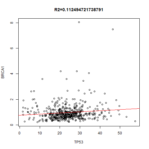
上面是指定一个基因在不同的癌种里面,本次讲指定任意两个基因,在所有癌种里面找到correlation并作图!图如下:
十二
28
上面是指定一个基因在不同的癌种里面,本次讲指定任意两个基因,在所有癌种里面找到correlation并作图!图如下:
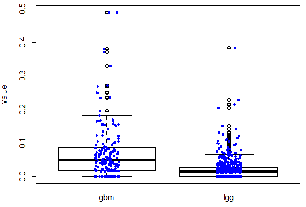
好像文章题目没有长度限制,太好了!本讲所实现的目标非常简单,如题,指定基因在不同癌种里面画boxplot,或者在所有的normal组织里面看表达量!下面是一个具体的例子:
下载IGV和导入文件的方法我就不多说了,可以直接在windows平台下使用,就跟你操作QQ一样,自己摸索就好了!
著名芬兰运动员Eero Mäntyranta,他拿过七枚奥运奖牌。他的血红细胞远超正常人水平,甚至一度被奥组委误以为服用了禁药。后来经过研究发现,他的EPOR基因上的一个位点rs121918116,发生了一个G>A的变异,使得他的血氧含量达到了普通人的150%,所以他耐力惊人。
在snpPedia里面可以查看这个位点的信息:http://snpedia.com/index.php/Rs121918116 Continue reading
我们在第19讲留下了一个悬念:为什么我算的染色体覆盖度与公司给我的报告不符合!!
公司算出每条染色体的覆盖度都接近于100%了,而我是结果是: Continue reading
前面我们在第8讲提到了公司给我的一个报告的统计表格,有人反映不会做。
本来应该只需要给我6亿条reads的(PE150测序,人30X),但是足足给了我8.9亿条!(但事实上很多paper发表的基因组高于60X的也不少)
表格里面提到了好几个概念,比如duplicate的reads,一般说的PCR造成的duplicate,在找变异的时候需要去除掉。然后是那些比对到了不同染色体的reads pair,虽然只有2.29% ,也是需要重点分析的。(前面我也讲了如何提取以及分别分析它们!) Continue reading
看来本次直播我的基因组分析流程效果还不错,不少朋友跟着自己动手开始分析全基因组测试数据了,值得表扬。其中有好几个朋友留言向我反映公司给的统计报告里面的覆盖度的问题,如下图: Continue reading
我博客里面有详细讲读原文查解去除PCR duplication的reads的原理和方法,还比较了samtools和picard这两个软件的区别,请点击阅看(仔细探究samtools的rmdup是如何行使去除PCR重复reads功能的),或者复制链接(http://www.bio-info-trainee.com/2003.html)到浏览器查看。 Continue reading
分析multiple mapping的情况,还是先用公司已经提供的bam文件来吧,后面我会用自己比对得到的bam文件再重新分析一次。
公司给我的bam数据是把有效测序数据通过 BWA(Li H et al.)比对到参考基因组 (b37),这是目前使用率很高的一个软件。在比对过程中,如果一个或一对 read(s) 在基因上可以有多个比对位置,BWA 的处理策略是从中选择一个最好的,如果有两个或以上最好的比对位置,则从中随机选择一个。这种多重比对(multiple hits)的处理对 SNP、INDEL 以及 CNV 等的检测有重要影响。 Continue reading
这类情况仅仅针对于双端测序数据,因为根据实验原理来看,对一个DNA片段,会把它的左右两端分别测序,但是测序仪器的测序长度有限,对本次实验来说,打断的DNA片段长度在350个碱基左右(这个长度只是一个分布,并不是真实值),理论来说测序是左右各150,加起来也就300,也就是说DNA片段中间还有50个碱基是测不到的(当然,实际上是有可能测通的)。而对这个配对的reads来说,来自于同一个DNA片段,所以理论上它们应该比对到同一条染色体的。也还是基于对sam格式的文件的理解,前面我们提到了sam文件的第3,7列指明了该reads比对到哪条染色体,以及该reads的配对reads比对到了哪条染色体(如果比对到同一条染色体,那么第7列是=符号)。所以我们只需要写脚本来提取即可! Continue reading
之前我们说了比对上的数据,那么会有人想到有没有没有比对上的数据呢?
既然是从我的血液里面提取到的DNA进行测序的,那么理论上测序仪出来的所有测序reads都应该是我的,也应该都可以比对到人类的参考基因组,但是实际过程中的确存在着未必对上的数据。
现有人类基因组毕竟只是个参考,也许我有某些独特的DNA序列呢?而且也不一定测序数据就都是人类的,也许我血液里面会有那么些微不纯粹呢?也有可能是某些片段变异的太多了,超过了常见的比对软件的承受能力,可以试用SHRIMP这个软件来提取一下。当然,这不是本讲的重点。 Continue reading
昨天,我们了解了一下SAM格式的比对结果,不知道大家理解的怎么样。但是全基因组测序数据实在是太大了,即使比对后把sam文件压缩成二进制的bam文件也还有55G(如何压缩转换可查看直播十二),如果完整的导入IGV查看会略微考验计算机配置。
比对工具到现在已经多如牛毛了,见列表: https://en.wikipedia.org/wiki/List_of_sequence_alignment_software 。但是能被大多数人熟知的,就是bowtie和bwa(我们在十一讲中用的才是bwa),它们把测序数据比对到参考基因组之后,都会生成一个sam格式的文件。随后的大部分分析都是基于sam格式进行的分析,虽然Jimmy多次强调这些基础知识的重要性需要大家私下自学。但是由于这个sam文件实在是太重要了!!!所以,不得不亲自抽出一讲来说说它,后面也会基于此写十多篇文章: Continue reading
熟悉GSEA软件的都知道,它只需要GCT,CLS和GMT文件,其中GMT文件,GSEA的作者已经给出了一大堆!就是记录broad的Molecular Signatures Database (MSigDB) 已经收到了18026个geneset,但是我奇怪的是里面竟然没有包括cancer testis的gene set,MSigDB的确是多,但未必全,其实里面还有很多重复。而且有不少几乎没有意义的gene set。那我想做自己的gene set来用gsea软件做分析,就需要自己制造gmt格式的数据。因为即使下载了MSigDB的gene set,本质上就是gmt格式的数据而已:http://software.broadinstitute.org/cancer/software/gsea/wiki/index.php/Data_formats#GMT:_Gene_Matrix_Transposed_file_format_.28.2A.gmt.29 Continue reading
这个也是读者来信最多的,关于基因组某些区域的起始终止坐标的下载问题,genomic feature的问题,一般是gtf文件或者bed文件,比如人类hg19上面的所有外显子的坐标记录文件,所有基因的坐标记录文件,所有lncRNA,rRNA等等,我这里拿CpG Islands记录文件下载的4种方式举例子给大家说明一下: Continue reading
这本是我为论坛的基础板块写的一个基础知识点,但是浏览量实在有限,不忍它蒙尘,特在博客重新发布一次!原帖见:http://www.biotrainee.com/thread-511-1-1.html
gene symbol 是非常官方的,由HUGO 组织负责维护,有专门的数据库HGNC database of human gene names | HUGO
以前分析数据的时候,有一些基因的symbol很奇怪,让我百思不得其解,比如
C orf 系列基因,
HS.系列基因,
KRTAP系列基因,
LOC系列基因,
MIR系列基因,
LINC系列基因
它们往往一个系列,就有好几百个基因;
C12orf44; Chromosome 12 Open Reading Frame 44; 这个是C orf系列基因的意思
MIR系列基因应该是 miRNA相关的基因
LINC系列基因应该就是long intergenic non-protein coding RNA
LOC系列基因,是非正式的,推定的,日后可能被更合适的名字替代
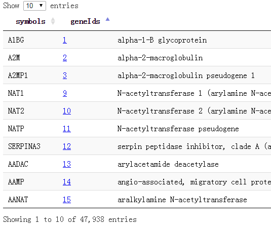
我这里做好了所有的基因对应关系,去生信菜鸟团QQ群里下载吧,共47938个基因的symbol和entrez gene id还有name,还有alias的对应!
还有一些RNA基因,根本就没有symbol,比如:CTA/B/C/D系列的
Aliases for ENSG00000271971 Gene
Quality Score for this RNA gene is 1
Aliases for ENSG00000271971 Gene
CTD-2006H14.2 5
External Ids for ENSG00000271971 Gene
Ensembl: ENSG00000271971
还有,如果你看到HS.开头的基因,它是unigene的ID了,已经不再是symbol啦。
这是系列文章,请先看:
ncbi现有的GPL已经过万了,但是bioconductor的芯片注释包不到一千,虽然bioconductor可以解决我们大部分的需要,比如affymetrix的95,133系列,深圳1.0st系列,HTA2.0系列,但是如果碰到比较生僻的芯片,bioconductor也不会刻意为之制作一个bioconductor的包,这时候就需要自行下载NCBI的GPL信息了,也可以通过R来解决:
##本质上是下载一个文件,读进R里面,然后解析行列式,得到芯片探针与基因的对应关系,看下面的代码,你就能理解了。 Continue reading

昨天我们说到,测序得到的fastq文件map到基因组之后,我们通常会得到一个sam或者bam为扩展名的文件。SAM的全称是sequence alignment/map format,而BAM就是SAM的二进制文件。通常sam文件太大,我们会生成bam文件来节省空间。sam文件和bam文件的转换用samtools这个软件就可以完成。 Continue reading