21

用R语言批量做T检验

需要做T检验的的数据如下:其中加粗加黑的是case,其余的是control,需要进行检验的是

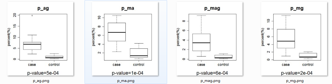
p_ma    p_mg    p_ag    p_mag 这四列数据,在case和control里面的差异,当然用肉眼很容易看出,control要比case高很多


individual m a g ma mg ag mag p_ma p_mg p_ag p_mag
HBV10-1 33146 3606 2208 308 111 97 39 0.79% 0.29% 0.25% 0.10%
HBV15-1 23580 10300 3140 1469 598 560 323 4.19% 1.71% 1.60% 0.92%
HBV3-1 107856 26445 15077 4773 2383 1869 1130 3.34% 1.67% 1.31% 0.79%
HBV4-1 32763 6448 4384 579 291 295 124 1.35% 0.68% 0.69% 0.29%
HBV6-1 122396 6108 7953 911 796 347 144 0.67% 0.59% 0.26% 0.11%
IGA-1 31337 22167 14195 3851 2752 4101 2028 6.50% 4.65% 6.92% 3.42%
IGA-10 6713 9088 12801 2275 2470 4284 1977 10.54% 11.44% 19.85% 9.16%
IGA-11 61574 23622 15076 5978 4319 3908 2618 6.71% 4.84% 4.38% 2.94%
IGA-12 38510 23353 20148 6941 6201 6510 4328 10.38% 9.27% 9.73% 6.47%
IgA-13 155379 81980 65315 26055 20085 17070 10043 10.38% 8.00% 6.80% 4.00%
IgA-14 345430 86462 71099 27541 21254 10923 6435 6.06% 4.67% 2.40% 1.42%
IgA-15 3864 3076 1942 378 207 389 145 4.66% 2.55% 4.80% 1.79%
IgA-16 3591 4106 2358 427 174 424 114 4.64% 1.89% 4.61% 1.24%
IgA-17 893 1442 799 68 28 78 18 2.27% 0.94% 2.61% 0.60%
IGA-2 23097 5083 5689 910 951 1173 549 2.89% 3.02% 3.72% 1.74%
IGA-3 14058 9364 8565 2130 1953 2931 1436 8.03% 7.36% 11.05% 5.41%
IGA-4 81571 36894 33664 11346 10131 9908 6851 8.86% 7.91% 7.74% 5.35%
IGA-5 27626 6492 4503 963 752 942 410 2.64% 2.06% 2.58% 1.12%
IGA-7 55348 5956 4028 833 476 468 207 1.30% 0.74% 0.73% 0.32%
IGA-8 31671 17097 10443 3894 2666 3514 2003 7.56% 5.17% 6.82% 3.89%


但是我们需要写程序对这些百分比在case和control里面进行T检验。

a=read.table("venn_dat.txt",header=T)

type=c(rep("control",5),rep("case",12),"control","control","case")

for (i in 9:12)

{

dat=as.numeric(unlist(lapply(a[i],function(x) strsplit(as.character(x),"%"))))

filename=paste(names(a)[i],".png",sep="")

png(file=filename, width = 320, height = 360)

b=t.test(dat~type)

txt=paste("p-value=",round(b$p.value[1],digits=4),sep="")

plot(as.factor(type),dat,ylab="percent(%)",main=names(a)[i],sub=txt,cex.axis=1.5,cex.sub=2,cex.main=2,cex.lab=1.5)

dev.off()

}

得到的图片如下:

image008

21

用R语言批量画韦恩图

需要画韦恩图的文件如下所示:

#CDR3_aa    count_all    count_IgM    count_IgA    count_IgG
CARGVDAGVDYW    243    25    196    22
CARHPRNYGNFDYW    174    171    3    0
CARENTMVRGVINPLDYW    166    8    75    83
CAREASDSISNWDDWYFDLW    129    15    114    0
CARDPDNSGAFDPW    118    1    117    0
CAKDLGGYW    98    3    4    91
CAREVADYDTYGWFLDLW    95    26    68    1
CVRNRGFFGLDIW    82    0    1    81
CARRSTNYHGWDYW    80    3    2    74

此处省略一万行。

简单解释一下数据,第一列是CDR3序列,我们需要对count_IgM    count_IgA    count_IgG这三列数据进行画韦恩图,数字大于0代表有,数字为0代表无。

这样我们根据序列就能得出每列数据所有的CDR3序列,即不为0的CDR3序列

每个个体都会输出一个统计文件,共20个文件需要画韦恩图

image005

对这个统计文件就可以进行画韦恩图。

画韦恩图的R代码如下:

library(VennDiagram)

files=list.files(path = ".", pattern = "type")

for (i in files){

a=read.table(i)

individual=strsplit(i,"\\.")[[1]][1]

image_name=paste(individual,".tiff",sep="")

IGM=which(a[,3]>0)

IGA=which(a[,4]>0)

IGG=which(a[,5]>0)

venn.diagram(list(IGM=IGM,IGA=IGA,IGG=IGG), fill=c("red","green","blue"), alpha=c(0.5,0.5,0.5), cex=2, cat.fontface=4, fontfamily=3, filename=image_name)

}

image007

但事实上,这个韦恩图很难表现出什么,因为我们的每个个体的count_IgM    count_IgA    count_IgG总数不一样。

19

Bioconductor系列之GenomicAlignments

Bioconductor系列包的安装方法都一样

source("http://bioconductor.org/biocLite.R")biocLite(“GenomicAlignments”)

这个包设计就是用来处理bam格式的比对结果的,具体功能非常多,其实还不如自己写脚本来做这些工作,更方便一点,实在没必要学别人的语法。大家有兴趣可以看GenomicAlignments的主页介绍,三个pdf文档来介绍。

http://www.bioconductor.org/packages/release/bioc/html/GenomicAlignments.html

我们首先读取示例pasillaBamSubset包带有的bam文件

library(pasillaBamSubset)

un1 <- untreated1_chr4()  # single-end reads

library(GenomicAlignments)

reads1 <- readGAlignments(un1)

查看reads1这个结果,可以看到把这个bam文件都读成了一个数据对象GAlignments object,

Bioconductor系列之GenomicAlignments632

readGAlignments这个函数就是读取我们bam文件的,生成的对象可以用多个函数来继续查看信息,比如它的列名都是函数

Seqnames(),strand(),cigar(),qwidth(),start(),end(),width(),njunc() 这些函数对这个GAlignments对象处理后会得到比对的各个情况的向量。

我们也可以读取这个GenomicAlignments包自带的bam文件,而不是pasillaBamSubset包带有的bam文件

> fls <- list.files(system.file("extdata", package="GenomicAlignments"),+                   recursive=TRUE, pattern="*bam$", full=TRUE)

> fls

[1] "C:/Program Files/R/R-3.1.2/library/GenomicAlignments/extdata/sm_treated1.bam"  [2] "C:/Program Files/R/R-3.1.2/library/GenomicAlignments/extdata/sm_untreated1.bam"

reads1 <- readGAlignments(fls[1])

比如我随意截图 cigar(reads1)的结果,就可以看出,大部分都是75M这样的比对情况,可以对这个向量进行统计完全匹配的情况,总共有6077总比对情况。

unique(cigar(reads1))

Bioconductor系列之GenomicAlignments1315

也可以用table格式来查看cigar,可以看到大部分都是M

head(cigarOpTable(cigar(reads1)))

Bioconductor系列之GenomicAlignments1385

接下来我们再读取PE测序数据的比对bam结果,看看分析方法有哪些。

Bioconductor系列之GenomicAlignments1422

U3.galp <- readGAlignmentPairs(untreated3_chr4(), use.names=TRUE, param=param0)head(U3.galp)

也可以分开查看左右两端测序数据的比对情况,跟上面的head是对应关系,上面的

[169,  205] -- [ 326,  362]在下面就被分成左右两个比对情况了。

> head(first(U3.galp))

GAlignments object with 6 alignments and 0 metadata columns:      seqnames strand       cigar    qwidth     start       end     width     njunc         <Rle>  <Rle> <character> <integer> <integer> <integer> <integer> <integer>  [1]     chr4      +         37M        37       169       205        37         0  [2]     chr4      +         37M        37       943       979        37         0  [3]     chr4      +         37M        37       944       980        37         0  [4]     chr4      +         37M        37       946       982        37         0  [5]     chr4      +         37M        37       966      1002        37         0  [6]     chr4      +         37M        37       966      1002        37         0  -------  seqinfo: 8 sequences from an unspecified genome

> head(last(U3.galp))

GAlignments object with 6 alignments and 0 metadata columns:      seqnames strand       cigar    qwidth     start       end     width     njunc         <Rle>  <Rle> <character> <integer> <integer> <integer> <integer> <integer>  [1]     chr4      -         37M        37       326       362        37         0  [2]     chr4      -         37M        37      1086      1122        37         0  [3]     chr4      -         37M        37      1119      1155        37         0  [4]     chr4      -         37M        37       986      1022        37         0  [5]     chr4      -         37M        37      1108      1144        37         0  [6]     chr4      -         37M        37      1114      1150        37         0  -------  seqinfo: 8 sequences from an unspecified genome

用isProperPair可以查看pe测序数据比对情况的,哪些没有配对比对成功

> table(isProperPair(U3.galp))FALSE  TRUE 29518 45828

还可以用Rsamtools包对我们的bam文件进行统计,看下面的代码中fls[1]和un1都是上面得到的bam文件全路径。

> library(Rsamtools)

> quickBamFlagSummary(fls[1], main.groups.only=TRUE)

group |    nb of |    nb of | mean / max                                   of |  records |   unique | records per                              records | in group |   QNAMEs | unique QNAMEAll records........................ A |     1800 |     1800 |    1 / 1  o template has single segment.... S |     1800 |     1800 |    1 / 1  o template has multiple segments. M |        0 |        0 |   NA / NA      - first segment.............. F |        0 |        0 |   NA / NA      - last segment............... L |        0 |        0 |   NA / NA      - other segment.............. O |        0 |        0 |   NA / NA Note that (S, M) is a partitioning of A, and (F, L, O) is a partitioning of M.Indentation reflects this.

> library(Rsamtools)

> quickBamFlagSummary(un1, main.groups.only=TRUE)

group |    nb of |    nb of | mean / max                                   of |  records |   unique | records per                              records | in group |   QNAMEs | unique QNAMEAll records........................ A |   204355 |   190770 | 1.07 / 10  o template has single segment.... S |   204355 |   190770 | 1.07 / 10  o template has multiple segments. M |        0 |        0 |   NA / NA      - first segment.............. F |        0 |        0 |   NA / NA      - last segment............... L |        0 |        0 |   NA / NA      - other segment.............. O |        0 |        0 |   NA / NA Note that (S, M) is a partitioning of A, and (F, L, O) is a partitioning of M.Indentation reflects this.


下面讲最后一个综合应用

biocLite("RNAseqData.HNRNPC.bam.chr14")

#这是一个665.5MB的RNA-seq测序数据的比对结果

library(RNAseqData.HNRNPC.bam.chr14)bamfiles <- RNAseqData.HNRNPC.bam.chr14_BAMFILESnames(bamfiles)  # the names of the runslibrary(Rsamtools)quickBamFlagSummary(bamfiles[1], main.groups.only=TRUE)flag1 <- scanBamFlag(isFirstMateRead=TRUE, isSecondMateRead=FALSE,                     isDuplicate=FALSE, isNotPassingQualityControls=FALSE)param1 <- ScanBamParam(flag=flag1, what="seq") #这里是设置readGAlignments的读取参数library(GenomicAlignments)gal1 <- readGAlignments(bamfiles[1], use.names=TRUE, param=param1)

mcols(gal1)$seqoqseq1 <- mcols(gal1)$seqis_on_minus <- as.logical(strand(gal1) == "-")oqseq1[is_on_minus] <- reverseComplement(oqseq1[is_on_minus])

这样就还原得到了原始测序数据啦!

18

Bioconductor系列之biomaRt

biomaRt是一个超级网络资源库,里面的信息非常之多,就是网页版的biomaRt的R语言接口。谷歌搜索 the biomart user’s guide filetype:pdf 这个关键词,就看到关于这个包的详细介绍以及例子,我这里简单总结一下它的用法。

这个包一直在更新,函数总是变化,而且需要联网才能使用,基本上等于废物一个,希望大家不要使用它~

包的安装

Continue reading

18

R语言DESeq找差异基因

一:安装并加装该R包

安装就用source("http://bioconductor.org/biocLite.R") ;biocLite("DESeq")即可,如果安装失败,就需要自己下载源码包,然后安装R模块。


二.所需要数据

它的说明书指定了我们一个数据

source("http://bioconductor.org/biocLite.R") ;biocLite("pasilla")

安装了pasilla这个包之后,在这个包的安装目录就可以找到一个表格文件,就是我们的DESeq需要的文件。

C:\Program Files\R\R-3.2.0\library\pasilla\extdata\pasilla_gene_counts.tsv

说明书原话是这样的

The table cell in the i-th row and the j-th column of the table tells how many reads have been mapped to gene i in sample j.

一般我们需要用htseq-count这个程序对我们的每个样本的sam文件做处理计数,并合并这样的数据

下面这个是示例数据,第一列是基因ID号,后面的每一列都是一个样本。

图片1

de = newCountDataSet( pasillaCountTable, condition )  #根据我们的样本因子把基因计数表格读入成一个cds对象,这个newCountDataSet函数就是为了构建对象!

对我们构建好的de对象就可以直接开始找差异啦!非常简单的几步即可

de=estimateSizeFactors(de)

de=estimateDispersions(de)

res=nbinomTest(de,"K","W") #最重要的就是这个res表格啦!

uniq=na.omit(res)

我这里是对4个样本用htseq计数后的文件来做的,贴出完整代码吧

library(DESeq)

#首先读取htseq对bam或者sam比对文件的计数结果

K1=read.table("742KO1.count",row.names=1)

K2=read.table("743KO2.count",row.names=1)

W1=read.table("740WT1.count",row.names=1)

W2=read.table("741WT2.count",row.names=1)

data=cbind(K1,K2,W1,W2)

data=data[-c(43630:43634),]

#把我们的多个样本计数结果合并起来成数据框,列是不同样本,行是不同基因

colnames(data)=c("K1","K2","W1","W2")

type=rep(c("K","W"),c(2,2))

#构造成DESeq的对象,并对分组样本进行基因表达量检验

de=newCountDataSet(data,type)

de=estimateSizeFactors(de)

de=estimateDispersions(de)

res=nbinomTest(de,"K","W")

#res就是我们的表达量检验结果

library(org.Mm.eg.db)

tmp=select(org.Mm.eg.db, keys=res$id, columns="GO", keytype="ENSEMBL")

ensembl_go=unlist(tapply(tmp[,2],as.factor(tmp[,1]),function(x) paste(x,collapse ="|"),simplify =F))

#首先输出所有的计数数据,加上go注释信息

all_res=res

res$go=ensembl_go[res$id]

write.csv(res,file="all_data.csv",row.names =F)

#然后输出有意义的数据,即剔除那些没有检测到表达的基因

uniq=na.omit(res)

sort_uniq=uniq[order(uniq$padj),]

write.csv(sort_uniq,file="sort_uniq.csv",row.names =F)

#然后挑选出padj值小于0.05的差异基因数据来做富集,富集用的YGC的两个包,在我前面的博客已经详细说明了!

tmp=select(org.Mm.eg.db, keys=sort_uniq[sort_uniq$padj<0.05,1], columns="ENTREZID", keytype="ENSEMBL")

diff_ENTREZID=tmp$ENTREZID

require(DOSE)

require(clusterProfiler)

diff_ENTREZID=na.omit(diff_ENTREZID)

ego <- enrichGO(gene=diff_ENTREZID,organism="mouse",ont="CC",pvalueCutoff=0.01,readable=TRUE)

ekk <- enrichKEGG(gene=diff_ENTREZID,organism="mouse",pvalueCutoff=0.01,readable=TRUE)

write.csv(summary(ekk),"KEGG-enrich.csv",row.names =F)

write.csv(summary(ego),"GO-enrich.csv",row.names =F)


05

国外最出名的R语言大会-useR

这是2014年的会议报告以及ppt,但是好像很多ppt都是需要翻墙才能下载

http://user2014.stat.ucla.edu/#tutorials

Morning Tutorials Monday, 9:15

Room Presenter Title
Palisades Salon A+B Max Kuhn Applied Predictive Modeling in R
Palisades Salon C+F Winston Chang Interactive graphics with ggvis
Palisades Salon D+E Yihui Xie Dynamic Documents with R and knitr [Slides] [Examples]
Hermosa Romain Francois C++ and Rcpp11 for beginners [slides]
Venice Bob Muenchen Managing Data with R
Sproul-Landing building, 3rd floor Matt Dowle Introduction to data.table [Tutorial] [Talk]
Sproul-Landing building, 4th floor Virgilio Gomez Rubio Applied Spatial Data Analysis with R
Sproul-Landing building, 5th floor Martin Morgan Bioconductor

Afternoon Tutorials Monday, 14:00

Room Presenter Title
Palisades Salon A+B Hadley Wickham Data manipulation with dplyr
Palisades Salon C+F Garrett Grolemund Interactive data display with Shiny and R
Palisades Salon D+E Drew Schmidt Programming with Big Data in R
Hermosa S繪ren H繪jsgaard Graphical Models and Bayesian Networks with R
Venice John Nash Nonlinear parameter optimization and modeling in R [slides]
Sproul-Landing building, 3rd floor Dirk Eddelbuettel An Example-Driven Hands-on Introduction to Rcpp [slides]
Sproul-Landing building, 4th floor Ramnath Vaidyanathan Interactive Documents with R
Sproul-Landing building, 5th floor Thomas Petzoldt Simulating differential equation models in R


然后2015年的也要开始了,有兴趣的朋友可以June 30 - July 3, 2015
Aalborg, Denmark看看,有很多干货分享!

http://user2015.math.aau.dk/#BN

2015的内容如下


01

ubuntu服务器解决方案第二讲-R程序包最新版的安装

发现自己搞服务器遇到的困难还是蛮多的,所以记录了一下,给菜鸟们指个路。
ubuntu对生信菜鸟来说是最好用的linux服务器,没有之一,因为它有apt-get。
首先,如果你的服务器里面有旧的R,那么删除Linux Ubuntu系统中原有的R软件包,代码如下:
sudo apt-get autoremove r-base-core # 删除系统中原有的R软件包
接下来,随便找到一个Ubuntu的软件源镜像
(http://mirror.bjtu.edu.cn/cran/bin/linux/ubuntu/ )
因为看我教程的大部分在国内,所以我拿北京大学举例子。
 当然,厦门大学也很赞,http://mirrors.xmu.edu.cn/CRAN/bin/linux/ubuntu/xenial/  不过,版本代号一定药搞清楚哦。
PS(2017/12/20, 没想到随便找到来一个,就挂掉了,唉:

厦门大学不再提供R语言镜像

)

Linux Ubuntu 12.04对应的名字是 precise,
ubuntu14.04,那么就应该是 trusty
ubuntu15.04 ,其代号为 vivid
Ubuntu 16.04 LTS,代号为Xenial Xerus(非洲的一种地松鼠),于UTC时间2016年4月21日正式发布。
比如我的Ubuntu 12.04就需要进入到 precise/目录,找到r-base-core相关的文件,发现有多个R的版本。
把这个软件源,增加到apt的sources.list文件中,代码如下:
deb http://mirror.bjtu.edu.cn/cran/bin/linux/ubuntu precise/
其余的ubuntu版本类似即可:
在/etc/apt/sources.list文件最下面,新加一行
~ sudo apt-get update # 更新源
~ sudo apt-get install r-base-core # 再次安装R语言软件包
~ R –version # 检查R的版本
这时我们就安装了最新的R语言版本—3.0.3版。
require(ggplot2)
Loading required package: ggplot2
Failed with error: ‘package ‘ggplot2’ was built before R 3.0.0: please re-install it’
这个失败原因是怎么回事?R 3.0.0 的问题吗?怎么解决?
R 2.x 升级 3.x 需要重新(编译)安装所有包:
update.packages(checkBuilt = TRUE, ask = FALSE)
当然如果你不是在R里面用install.package来安装包的话
你还需要
sudo apt-get install r-base-dev
这样你才能从源代码编译R的包
但是如果你导入的R源被你的服务器拒绝,你就惨了
The following signatures couldn't be verified because the public key is not
以下签名不能因为公钥未验证
16

转录组edgeR分析差异基因

转录组edgeR分析差异基因

edgeR是一个研究重复计数数据差异表达的Bioconductor软件包。一个过度离散的泊松模型被用于说明生物学可变性和技术可变性。经验贝叶斯方法被用于减轻跨转录本的过度离散程度,改进了推断的可靠性。该方法甚至能够用最小重复水平使用,只要至少一个表型或实验条件是重复的。该软件可能具有测序数据之外的其他应用,例如蛋白质组多肽计数数据。可用性:程序包在遵循LGPL许可证下可以从Bioconductor网站。

一:下载安装该软件

下载安装edgeR这个R包,因为这是一次讲R包的下载,我就啰嗦一点,这种生物信息学的包不同于普通的R包,是需要用biocLite来安装的,命令如下

转录组edgeR分析差异基因304


Continue reading

15

仿写fastqc软件的一些功能-R代码

仿写fastqc软件的一些功能(下)

文件来自于上面perl代码的输出文件,好像算法有点问题,26G的文件居然处理近一个小时才出数据!

仿写fastqc软件的一些功能-下-R代码263

R语言本身自带的画图工具都很丑,懒得说了,可以用ggplot2来重新画一个,不是项目要求没有报酬我就懒得画了,大家面前看看画图原理即可。

Continue reading