14

R语言画网络图三部曲之sna

如果只是画网络图,那么只需要把所有的点,按照算好的坐标画出来,然后把所有的连线也画出即可!

其中算法就是,点的坐标该如何确定?Two of the most prominente algorithms (Fruchterman & Reingold’s force-directed placement algorithm and Kamada-Kawai’s)
有一个networkD3的包可以直接画图,但是跳过了确定点的坐标这个步骤,我重新找了一包,可以做到!
作者只是用sna包来得到数据,其实用的是ggplot来画网络图!
需要熟悉network包里面的network对象的具体东西,如何自己构造一个,然后数学sna包如何计算layout即可
解读这个包,也可以自己画网络图,代码如下:
plot(plotcord)
text(x=plotcord$X1+0.2,y=plotcord$X2,labels = LETTERS[1:10])
for (i in 1:10){
  for (j in 1:10){
    if(tmp[i,j]) lines(plotcord[c language="(i,j),1"][/c],plotcord[c language="(i,j),2"][/c])
  }
}
当然,我们还没有涉及到算法,就是如何生成plotcord这个坐标矩阵的!
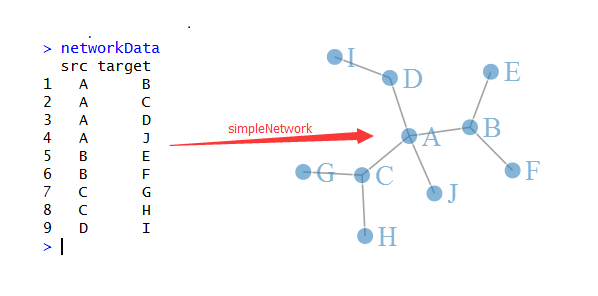
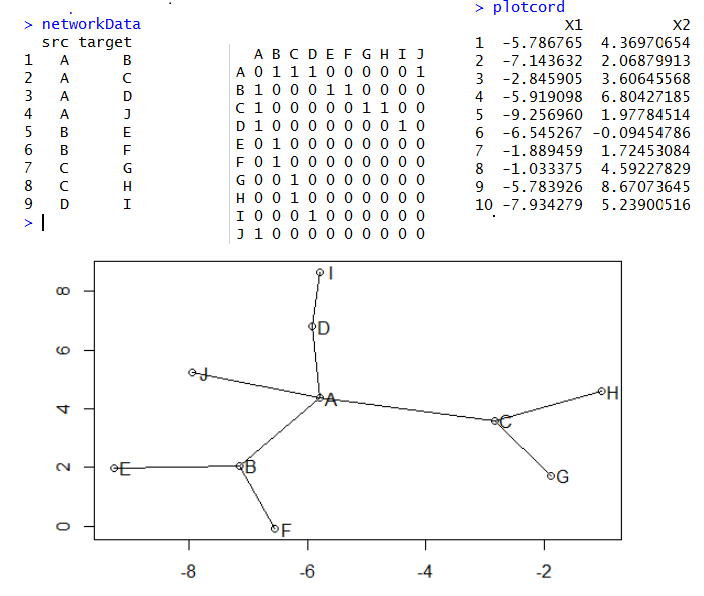
大家看下面这个示意图就知道网络图是怎么样画出来的了,首先我们有一些点,它们之间有联系,都存储在networData这个数据里面,是10个点,共9个连接,然后我用reshape包把它转换成连接矩阵,理论上10个点的两两相互作用应该有100条线,但是我们的数据清楚的说明只有9条,所以只有9个1,其余的0代表点之间没有关系。接下来我们用sna这个包对这个连接矩阵生成了这10个点的坐标(这个是重点),最后很简单了,把点和线画出来即可!
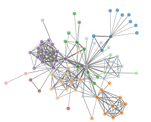
1

另外一个例子:
net=network(150, directed=FALSE, density=0.03)
m <- as.matrix.network.adjacency(net) # get sociomatrix  
# get coordinates from Fruchterman and Reingold's force-directed placement algorithm.
plotcord <- data.frame(gplot.layout.fruchtermanreingold(m, NULL)) 
# or get it them from Kamada-Kawai's algorithm: 
# plotcord <- data.frame(gplot.layout.kamadakawai(m, NULL)) 
colnames(plotcord) = c("X1","X2")  ###所有点的坐标,共150个点
edglist <- as.matrix.network.edgelist(net) ##所有点之间的关系-edge ##共335条线
edges <- data.frame(plotcord[edglist[,1],], plotcord[edglist[,2],]) ##两点之间的连线的具体坐标,335条线的起始终止点点坐标
原始代码如下:
library(network)
library(ggplot2)
library(sna)
library(ergm)
clipboard
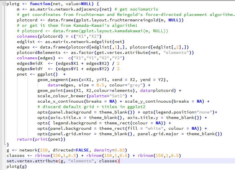
大家可以试用这个代码,因为它用的ggplot,肯定比我那个简单R作图要好看多了
参考算法文献:


14

R语言画网络图三部曲之networkD3

首先,我们需要了解一下基础知识:
网络图是为了展示数据与数据之间的联系,在生物信息学领域,一般是基因直接的相互作用关系,或者通路之间的联系!
通俗点说,就是我有一些点,它们之间并不是两两相互联系,而是有部分是有连接的,那么我应该如何把这些点画在图片上面呢?因为这些都并没有X,Y坐标,只有连接关系,所以我们要根据一个理论来给它们分配坐标,这样就可以把它们画出来了,然后也可以对这些点进行连线,连完线后,就是网络图啦!!!
而给它们分配坐标的理论有点复杂,大概类似于物理里面的万有引力和洛仑磁力相结合来给它们分配一个位置,使得总体的能量最小,就是最稳定状态!而通常这个状态是逼近,而不是精确,所以我们其实对同样的数据可以画出无数个网络图,只需使得网络图合理即可!
看这个ppt:http://statmath.wu.ac.at/research/friday/resources_WS0708_SS08/igraph.pdf

基本上就都理解了
画网络图真的好复杂呀!!!
大部分人都是用D3JS来画图:http://bl.ocks.org/mbostock/2706022
一步步讲受力分析图是如何画的:https://github.com/mbostock/d3/wiki/Force-Layout

接下来, 我们直接看看R里面是如何画网络图的,我们首推一个包:networkD3/

这个包非常好用,只需要做好data,然后用它提供的几个函数即可!
重要的是熟悉输入数据是什么,还可以结合shinny包来展示数据,非常好用!!!
具体怎么安装这个R包,我就不讲了,它的github主页上面其实也有说明书,很容易看懂的
最简单的用法,就是构造一个联结矩阵,把所有的连接关系都存储起来,然后直接用一个函数就可以画图啦!
# Plot
library(networkD3)
simpleNetwork(networkData,fontSize=25)
可以看出网络图,就是把所有的点,按照算好的坐标画出来,然后把所有的连线也画出即可!
其中算法就是,点的坐标该如何确定?Two of the most prominente algorithms (Fruchterman & Reingold’s force-directed placement algorithm and Kamada-Kawai’s)

clipboard

但是这个软件有一个弊端就是,生成图片之后,并没有给出这些点的坐标,当然,这种坐标基本上也很少有人需要,可视化就够了!
如果这些点还分组了,而且连接还有权重,那么网络图就复杂一点,比如下面这个:
就不仅仅是需要提供所有的link的信息,link还多了一列,是value,而且还需提供所有的node信息,node多了一列是分组。
clipboard
当然,还有好几个图,大家可以自己慢慢用,自己体会!
sankeyNetwork
sankeyNetwork
radialNetwork
diagonalNetwork
dendroNetwork
也可以把生成的网络图直接保存成网页,动态显示!
14

用broad出品的软件来处理bam文件几次遇到文件头错误

报错如下:ERROR MESSAGE: SAM/BAM file input.marked.bam is malformed: SAM file doesn't have any read groups defined in the header.  The GATK no longer supports SAM files without read groups !

有些人遇到的是bam的染色体顺序不一样,还有可能是染色体的名字不一样,比如>1和>chr1的区别,虽然很傻,但是遇到这样问题的还不少!
还有一些人是遇到基因组没有dict文件,也是用picard处理一下就好。

大部分人是在GATK遇到的,我是在RNA-SeQC遇到的,不过原理都是一样的。
都是因为做alignment的时候并未添加头信息,比如:
bwa samse ref.fa my.sai my.fastq > my.sam
samtools view -bS my.sam > my.bam
samtools sort my.bam my_sorted
java -jar ReordereSam.jar I=/path/my_sorted.bam O=/path/my_reordered.bam R=/path/ref.fa
通过这个代码可以得到排序好的bam,但是接下来用GATK就会报错
java -jar GenomeAnalysisTK.jar -T DepthOfCoverage -R /paht/ref.fa -I /path/aln_reordered.bam
就是因为没有头信息,group相关信息,解决方法有两种:
bwa samse -r @RG\tID:IDa\tSM:SM\tPL:Illumina ref.fa my.sai my.fastq > my.sam
java -jar AddOrReplaceReadGroups I=my.bam O=myGr.bam LB=whatever PL=illumina PU=whatever SM=whatever
一种是比对的时候就加入头信息,这个需要比对工具的支持。
第二种是用picard工具来修改bam,推荐用这个!虽然我其实并不懂这些头文件信息是干嘛的, 但是broad开发的软件就是需要!希望将来去读PHD能系统性的学习一些基础知识!


14

用RNA-SeQC得到表达矩阵RPKM值

这个软件不仅仅能做QC,而且可以统计各个基因的RPKM值!尤其是TCGA计划里面的都是用它算的
一、程序安装
直接在官网下载java版本软件即可使用:http://www.broadinstitute.org/cancer/cga/tools/rnaseqc/RNA-SeQC_v1.1.8.jar
但是需要下载很多注释数据
clipboard

二、输入数据

clipboard

箭头所指的文件,一个都不少,只有那个rRNA.tar我没有用, 因为这个软件有两种使用方式,我用的是第一种
三、软件使用
软件的官网给力例子,很容易学习:
RNA-SeQC can be run with or without a BWA-based rRNA level estimation mode. To run without (less accurate, but faster) use the command:
java -jar RNASeQC.jar -n 1000 -s "TestId|ThousandReads.bam|TestDesc" -t gencode.v7.annotation_goodContig.gtf -r Homo_sapiens_assembly19.fasta -o ./testReport/ -strat gc -gc gencode.v7.gc.txt 
我用的就是这个例子,这个例子需要的所有文件里面,染色体都是没有chr的,这个非常重要!!!
代码如下:
 java -jar RNA-SeQC_v1.1.8.jar  \
-n 1000 \
-s "TestId|ThousandReads.bam|TestDesc" \
-t gencode.v7.annotation_goodContig.gtf \
-r ~/ref-database/human_g1k_v37/human_g1k_v37.fasta  \
-o ./testReport/ \
-strat gc \
-gc gencode.v7.gc.txt \
To run the more accurate but slower, BWA-based method :
java -jar RNASeQC.jar -n 1000 -s "TestId|ThousandReads.bam|TestDesc" -t gencode.v7.annotation_goodContig.gtf -r Homo_sapiens_assembly19.fasta -o ./testReport/ -strat gc -gc gencode.v7.gc.txt -BWArRNA human_all_rRNA.fasta
Note: this assumes BWA is in your PATH. If this is not the case, use the -bwa flag to specify the path to BWA
四、结果解读
运行要点时间,就那个一千条reads的测试数据都搞了10分钟!
出来一大堆突变,具体解释,官网上面很详细,不过,比较重要的当然是RPKM值咯,还有QC的信息
clipboard
TCGA数据里面都会提供由RNA-SeQC软件处理得到的表达矩阵!
Expression
  • RPKM data are used as produced by RNA-SeQC.
  • Filter on >=10 individuals with >0.1 RPKM and raw read counts greater than 6.
  • Quantile normalization was performed within each tissue to bring the expression profile of each sample onto the same scale.
  • To protect from outliers, inverse quantile normalization was performed for each gene, mapping each set of expression values to a standard normal.
软件的主页是:


14

华盛顿大学把所有的变异数据都用自己的方法注释了一遍,然后提供下载

华盛顿大学把所有的变异数据都用自己的方法注释了一遍,然后提供下载:
文献是:Kircher M, Witten DM, Jain P, O'Roak BJ, Cooper GM, Shendure J. 

A general framework for estimating the relative pathogenicity of human genetic variants.
Nat Genet. 2014 Feb 2. doi: 10.1038/ng.2892.
PubMed PMID: 24487276.

文中的观点是:现在大多的变异数据注释方法都非常单一,通常是看看该位点是否保守,对蛋白功能的改变,在什么domain上面等等。
但这样是远远不够的,所以他们提出了一个新的注释方法,用他们自己的CADD方法把现存的一些公共数据库的变异位点(约86亿的位点)都注释了一下,并对每个位点进行了打分。
C scores correlate with allelic diversity, annotations of functionality, pathogenicity, disease severity, experimentally measured regulatory effects and complex trait associations, and they highly rank known pathogenic variants within individual genomes.
总之,他们的方法是无与伦比的!
所有他们已经注释好的数据下载地址是:http://cadd.gs.washington.edu/download
这些数据在很多时候非常有用,尤其是想跟自己得到的突变数据做交叉验证,或者做一下统计分析的时候!
clipboard
人的基因组才300亿个位点,他们就注释了86亿!!!
所以有三百多G的压缩包数据,我想,一般的公司或者单位都不会去用这个数据了!
14

蛋白质相互作用(PPI)数据库大全

最近遇到一个项目需要探究一个gene list里面的基因直接的联系,所以就想到了基因的产物蛋白的相互作用关系数据库,发现这些数据库好多好多!
一个比较综合的链接是:A compendium of PPI databases can be found in http://www.pathguide.org/.

里面的数据库非常多,仅仅是对于人类就有

Your search returned 207 results in 9 categories with the following search parameters:

人类的六个主要PPI是:Analysis of human interactome PPI data showing the coverage of six major primary databases (BIND, BioGRID, DIP, HPRD, IntAct, and MINT), according to the integration provided by the meta-database APID.
BIND the biomolecular interaction network database died link
DIP the database of interacting proteins http://dip.doe-mbi.ucla.edu/ 
MINT the molecular interaction database http://mint.bio.uniroma2.it/mint/ 
STRING Search Tool for the Retrieval of Interacting Genes/Proteins http://string-db.org/  
HPRO Human protein reference database http://www.hprd.org/ 
BioGRID The Biological General Repository for Interaction Datasets http://thebiogrid.org/ 
这些数据库大部分都还有维护者,还在持续更新,每次更新都可以发一篇paper,而数据库收集的paper引用一般都上千,如果你做了一个数据库,才十几个人引用,那就说明你是自己在跟自己玩。
其中比较好用的是宾夕法尼亚州匹兹堡的大学的一个:http://severus.dbmi.pitt.edu/wiki-pi/
(a) PPI definition; a definition of a protein-to-protein interaction compared to other biomolecular relationships or associations.
(b)PPI determination by two alternative approaches: binary and co-complex; a description of the PPIs determined by the two main types of experimental technologies.
(c) The main databases and repositories that include PPIs; a description and comparison of the main databases and repositories that include PPIs, indicating the type of data that they collect with a special distinction between experimental and predicted data.
(d) Analysis of coverage and ways to improve PPI reliability; a comparative study of the current coverage on PPIs and presentation of some strategies to improve the reliability of PPI data.
(e) Networks derived from PPIs compared to canonical pathways; a practical example that compares the characteristics and information provided by a canonical pathway and the PPI network built for the same proteins. Last, a short summary and guidance for learning more is provided.
现在的蛋白质相互作用数据库的数据都很有限,但是在持续增长,一般有下面四种原因导致数据被收录到数据库
There are four common approaches for PPI data expansions:
1) manual curation from the biomedical literature by experts;
2) automated PPI data extraction from biomedical literature with text mining methods;
3) computational inference based on interacting protein domains or co-regulation relationships, often derived from data in model organisms; and
4) data integration from various experimental or computational sources.
Partly due to the difficulty of evaluating qualities for PPI data, a majority of widely-used PPI databases, including DIP, BIND, MINT, HPRD, and IntAct, take a "conservative approach" to PPI data expansion by adding only manually curated interactions. Therefore, the coverage of the protein interactome developed using this approach is poor.
In the second literature mining approach, computer software replaces database curators to extract protein interaction (or, association) data from large volumes of biomedical literature . Due to the complexity of natural language processing techniques involved, however, this approach often generates large amount of false positive protein "associations" that are not truly biologically significant "interactions".
The challenge for the integrative approach is how to balance quality with coverage.
In particular, different databases may contain many redundant PPI information derived from the same sources, while the overlaps between independently derived PPI data sets are quite low .
参考:
2009年发表的HIPPI数据库:http://bmcgenomics.biomedcentral.com/articles/10.1186/1471-2164-10-S1-S16#CR6_2544 (是对HPRD [11], BIND [20], MINT [21], STRING [26], and OPHID数据库的整合)
14

居然可以下载千人基因组计划的所有数据bam,vcf数据

它有两个ftp站点存储所有的数据!
直接看最新版的数据,共有NA编号开头的1182个人,HG开头的1768个人!
每个人的目录下面都有 四个数据文件夹
Oct 01 2014 00:00    Directory alignment
Oct 01 2014 00:00    Directory exome_alignment
Oct 01 2014 00:00    Directory high_coverage_alignment
Oct 01 2014 00:00    Directory sequence_read
这些数据实在是太丰富了!
也可以直接看最新版的vcf文件,记录了这两千多人的所有变异位点信息!
可以直接看到所有的位点,具体到每个人在该位点是否变异!
不过它的基因型信息是通过MVNcall+SHAPEIT这个程序call出来的,具体原理见:http://www.ncbi.nlm.nih.gov/pubmed/23093610
clipboard