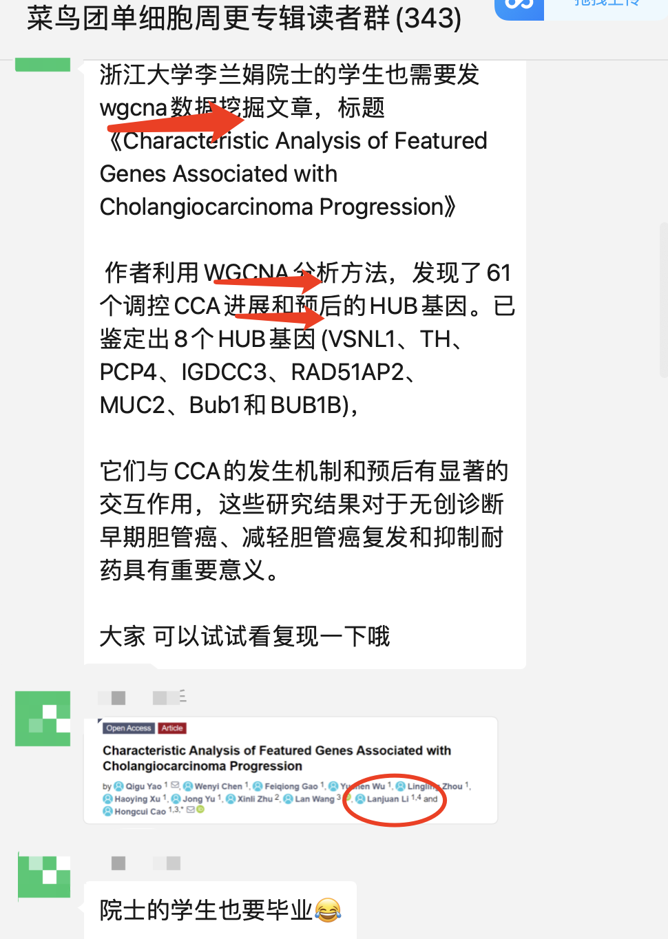
看到了交流群小伙伴分享了一系列数据挖掘文章,都是浙江大学李兰娟院士的学生的成果。其中一个《Characteristic Analysis of Featured Genes Associated with Cholangiocarcinoma Progression》倒是蛮简单的,挑选TCGA数据库里面的 GDC TCGA Bile Duct Cancer (CHOL)&removeHub=https%3A%2F%2Fxena.treehouse.gi.ucsc.edu%3A443) 数据集,然后根据里面的样品的二分类属性(肿瘤样品和正常组织对照)做一个简单的差异分析,然后基于差异分析后的基因列表进行go和kegg的数据库注释,以及使用WGCNA算法构建网络,然后挑选合适的网络看里面的hub基因而已。
我们分两步走,完成这个数据挖掘的复现。
首先是差异分析
挑选TCGA数据库里面的 GDC TCGA Bile Duct Cancer (CHOL)&removeHub=https%3A%2F%2Fxena.treehouse.gi.ucsc.edu%3A443) 数据集,然后根据里面的样品的二分类属性(肿瘤样品和正常组织对照)做一个简单的差异分析,表达量矩阵文件路径是;
有了这个文件,差异分析非常简单,也是分成3步走,代码如下所示:
首先是解析表达量矩阵
# 魔幻操作,一键清空
rm(list = ls())
options(stringsAsFactors = F)
library(data.table)
a1=fread( 'TCGA-CHOL.htseq_counts.tsv.gz' ,
 data.table = F)
dim(a1)
a1[1:4,1:4]
a1[(nrow(a1)-5):nrow(a1),1:4]
dim(a1)
# all data is then log2(x+1) transformed.

#length(unique(a1$AccID))
#length(unique(a1$GeneName))

mat= a1[,2:ncol(a1)]
mat[1:4,1:4]
mat=mat[1:(nrow(a1)-4),]
mat=ceiling(2^(mat)-1) #log2(x+1) transformed.
mat[1:4,1:4]

rownames(mat) = gsub('[.][0-9]+','',a1$Ensembl_ID[1:(nrow(a1)-4)])
keep_feature <- rowSums (mat > 1) > 1
colSums(mat)/1000000
table(keep_feature)
mat <- mat[keep_feature, ]
mat[1:4,1:4]
mat=mat[, colSums(mat)/1000000 >10]
dim(mat)
colnames(mat)
ensembl_matrix=mat
colnames(ensembl_matrix)
ensembl_matrix[1:4,1:4]
上面的表达量矩阵目前是ensembl数据库的id格式,不符合人类正常的阅读习惯,我们接下来需要进行简单的id转换
简单的id转换
library(AnnoProbe)
head(rownames(ensembl_matrix))
ids=annoGene(rownames(ensembl_matrix),'ENSEMBL','human')
head(ids)
ids=ids[!duplicated(ids$SYMBOL),]
ids=ids[!duplicated(ids$ENSEMBL),]
symbol_matrix= ensembl_matrix[match(ids$ENSEMBL,
 rownames(ensembl_matrix)),]

rownames(symbol_matrix) = ids$SYMBOL
#symbol_matrix = ensembl_matrix
symbol_matrix[1:4,1:4]
然后确定样品的分组后差异分析
library(stringr)
symbol_matrix[1:4,1:4]
colnames(symbol_matrix)
# group_list=ifelse( grepl('PLVX',colnames(symbol_matrix)),'control','case' )
group_list=ifelse(substring(colnames(symbol_matrix),14,15)=='11',
 'control','case' )
table(group_list)
group_list = factor(group_list,levels = c('control','case' ))
group_list
# save(symbol_matrix, group_list,
# file='symbol_matrix.Rdata')
# load( file='symbol_matrix.Rdata')
colnames(symbol_matrix)

save(symbol_matrix,group_list,file = 'symbol_matrix.Rdata')
前面的symbol_matrix和group_list制作成功后,两分组实验设计的转录组测序后的差异分析和富集分析都是无需修改的代码,默认跑一下即可:
source('scripts/step2-qc-counts.R')
source('scripts/step3-deg-deseq2.R')
source('scripts/step3-deg-edgeR.R')
source('scripts/step3-deg-limma-voom.R')
source('scripts/step4-qc-for-deg.R')
source('scripts/step5-anno-by-GSEA.R')
source('scripts/step5-anno-by-ORA.R')
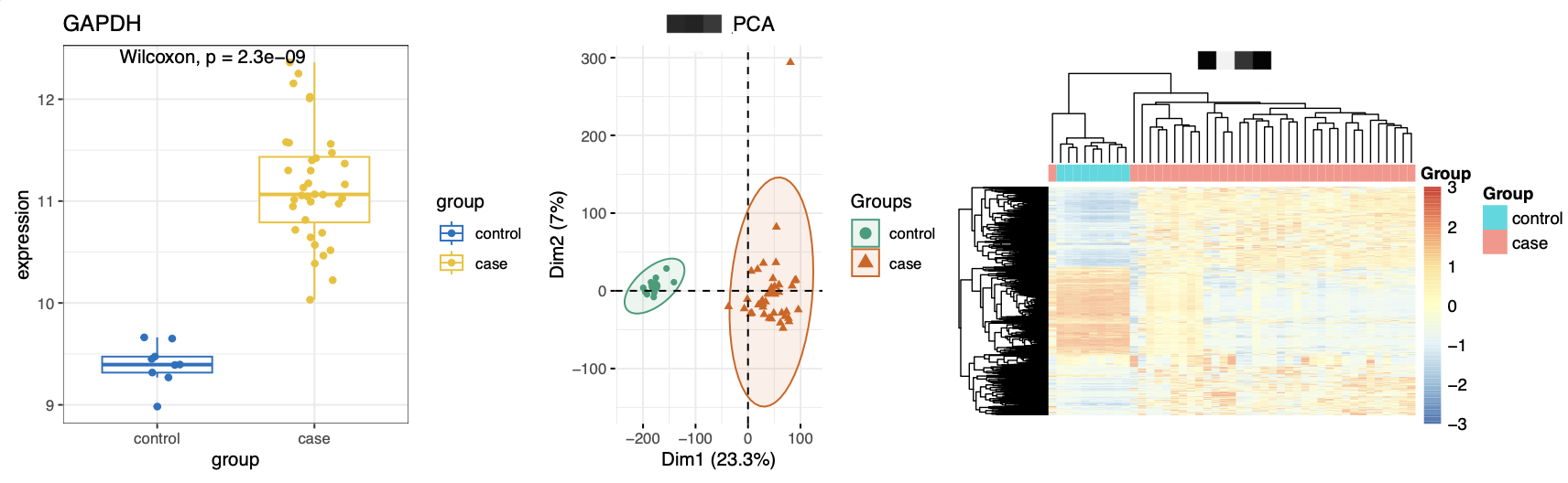
很简单的可以看到我们默认不会有表达量变化的GAPDH在这里居然也是很明显的差异基因,在肿瘤里面上调了 :
差异分析的结果也可以看到,上下调基因数量实在是太多了:
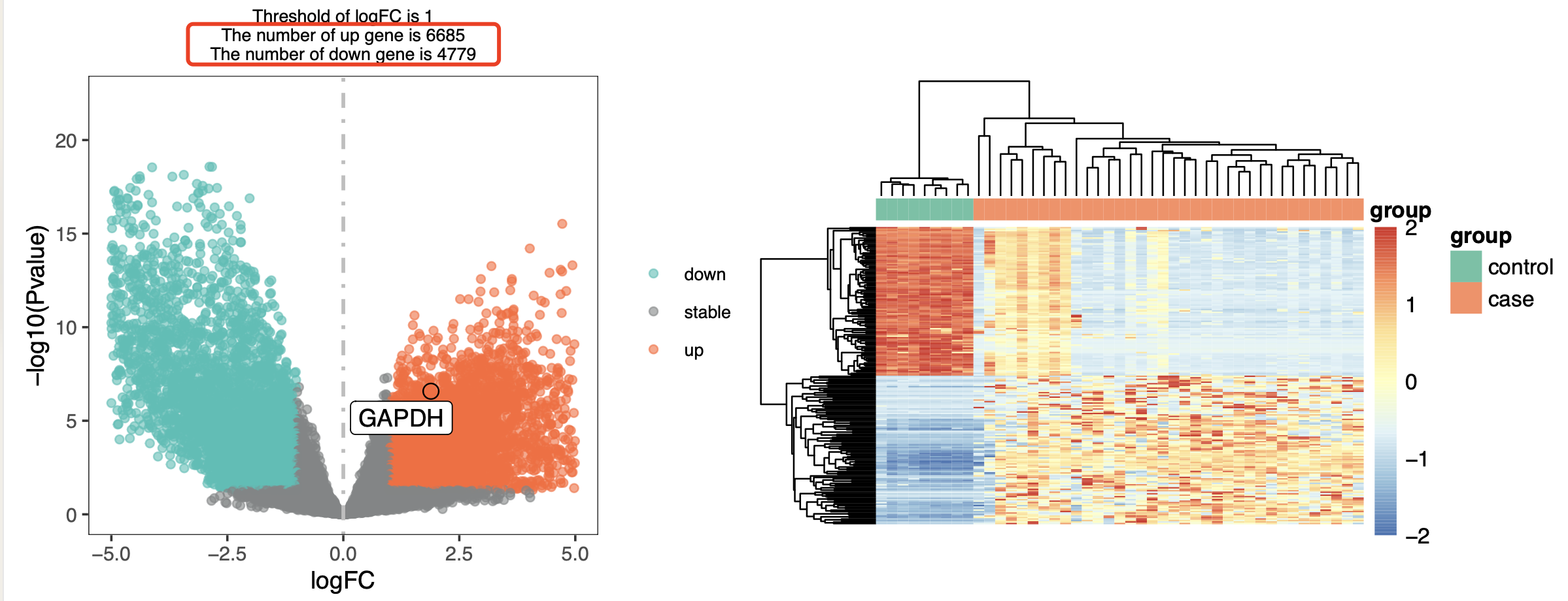
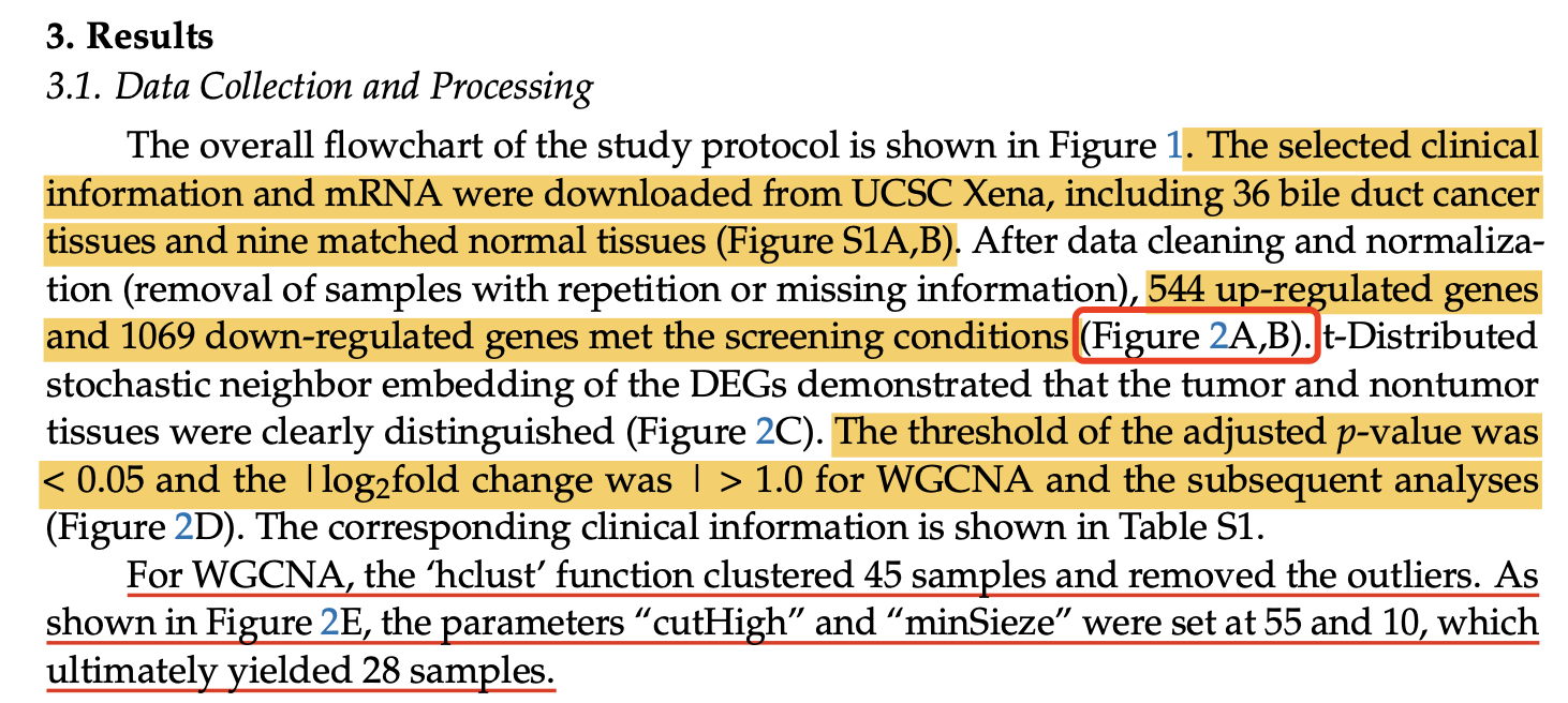
所以,我们的阈值必须变化,但是文章里面呢,Volcano plot of 1613 DEGs in between CCA patients and normal tissue (adjusted p-value < 0.05; |log2fold change| > 1) 很明显是有问题的,无论是使用什么样的转录组差异分析算法,都不太可能使用这样的阈值可以拿到这样的数据量的差异基因。
那么到底是问题出在哪里呢?我们的代码是公开的:
- https://cowtransfer.com/s/e1817982ce974c 点击链接查看 [ 2023-浙江大学李兰娟院士-WGCNA数据挖掘-step1-deg.zip ] ,或访问奶牛快传 cowtransfer.com 输入传输口令 uwiucz 查看;
感兴趣的小伙伴可以帮我们检查一下哦!
另外,预告一下,前面的差异基因拿到了之后,接下来我们要视频号直播wgcna数据分析过程啦。