最近七月份学徒们在集中做单细胞联系,其中一个学徒很不幸,拿到了单个10x样品的项目,纯粹的就是一个普通的黑色素瘤细胞系的测序,四千多个细胞而已。理论上是非常的均一,没办法跟以前的肿瘤研究的单细胞数据的第一次分群的通用规则:
- immune (CD45+,PTPRC),
- epithelial/cancer (EpCAM+,EPCAM),
- stromal (CD10+,MME,fibo or CD31+,PECAM1,endo)
所以我给他的建议是不管三七二十一,先分群,然后看每个亚群功能异质性,给出注释,并且给出临床生存分析结果。
首先你需要自己去GEO数据库里面下载 GSM4592552_filtered_gene_bc_matrices_h5.h5 文件,然后就可以follow我们的这个教程啦!
单细胞数据处理流程的前面的降维聚类分群超级简单了:
library(Seurat)
#读取单细胞数据,这里是h5文件
sce.all=CreateSeuratObject(Read10X_h5('GSM4592552_filtered_gene_bc_matrices_h5.h5'))
sce.all.filt=sce.all
sce.all.filt = FindVariableFeatures(sce.all.filt)
sce.all.filt = ScaleData(sce.all.filt,
vars.to.regress = c("nFeature_RNA", "percent_mito"))
sce.all.filt = RunPCA(sce.all.filt, npcs = 20)
sce.all.filt = RunTSNE(sce.all.filt, npcs = 20)
sce.all.filt = RunUMAP(sce.all.filt, dims = 1:20)
sce.all=sce.all.filt
sce.all <- FindNeighbors(sce.all, dims = 1:10)
sce.all <- FindClusters(sce.all, resolution = 0.2)
names(sce.all@reductions)
colnames(sce.all@meta.data)
colnames(sce.all@meta.data)
Idents(sce.all)="RNA_snn_res.0.2"
sce.all@active.ident
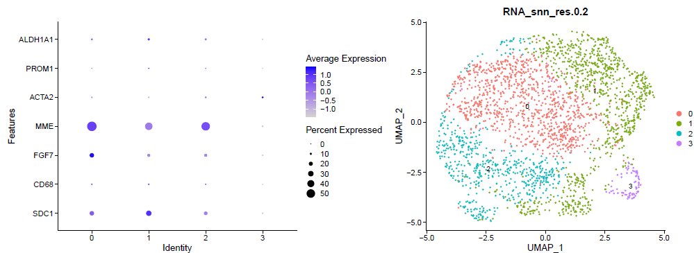
DimPlot(sce.all, reduction = "umap",label = T, )
ggsave('umap_by_seurat_clusters_res_0.2.png')
出图如下所示:
参考前面的例子:人人都能学会的单细胞聚类分群注释 ,我们演示了第一层次的分群。
如果你对单细胞数据分析还没有基础认知,可以看基础10讲:
- 01. 上游分析流程
- 02.课题多少个样品,测序数据量如何
- 03. 过滤不合格细胞和基因(数据质控很重要)
- 04. 过滤线粒体核糖体基因
- 05. 去除细胞效应和基因效应
- 06.单细胞转录组数据的降维聚类分群
- 07.单细胞转录组数据处理之细胞亚群注释
- 08.把拿到的亚群进行更细致的分群
- 09.单细胞转录组数据处理之细胞亚群比例比较
这个时候的每个亚群其实区分度还行啦,如果具体看每个亚群功能,就需要找到各自的高表达量基因,如下所示:
这个代码是:
table(Idents(sce))
sce.markers <- FindAllMarkers(object = sce, only.pos = TRUE, min.pct = 0.25,
thresh.use = 0.25)
DT::datatable(sce.markers)
pro='RNA_snn_res.0.2'
write.csv(sce.markers,file=paste0(pro,'_sce.markers.csv'))
library(dplyr)
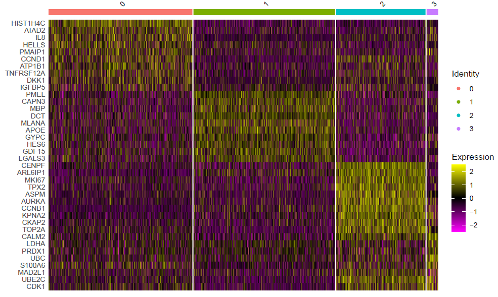
top10 <- sce.markers %>% group_by(cluster) %>% top_n(10, avg_log2FC)
DoHeatmap(sce,top10$gene,size=3)
ggsave(filename=paste0(pro,'_sce.markers_heatmap.pdf'))
library(dplyr)
top3 <- sce.markers %>% group_by(cluster) %>% top_n(3, avg_log2FC)
DoHeatmap(sce,top3$gene,size=3)
ggsave(paste0(pro,'DoHeatmap_check_top3_markers_by_clusters.pdf'))
p <- DotPlot(sce, features = unique(top3$gene),
assay='RNA' ) + coord_flip()
p
ggsave(paste0(pro,'DotPlot_check_top3_markers_by_clusters.pdf'))
save(sce.markers,file = 'sce.markers.Rdata')
但是各个亚群的基因数量太多, 仍然是肉眼看的累,如果生物学背景知识不够,很难说出个所以然,这个时候clusterProfiler的compareCluster函数就可以派上用场啦
load(file = 'sce.markers.Rdata')
table(sce.markers$cluster)
library(clusterProfiler)
library(org.Hs.eg.db)
library(ggplot2)
ids=bitr(sce.markers$gene,'SYMBOL','ENTREZID','org.Hs.eg.db')
sce.markers=merge(sce.markers,ids,by.x='gene',by.y='SYMBOL')
gcSample=split(sce.markers$ENTREZID, sce.markers$cluster)
gcSample # entrez id , compareCluster
xx <- compareCluster(gcSample, fun="enrichKEGG",
 organism="hsa", pvalueCutoff=0.05)
p=dotplot(xx)
p+ theme(axis.text.x = element_text(angle = 45,
 vjust = 0.5, hjust=0.5))
p

ggsave('compareCluster-sce.markers.pdf')
如下所示:
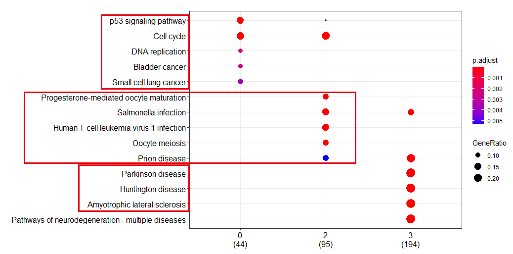
如果你还不知道clusterProfiler的compareCluster函数,赶快去看clusterProfiler4.0啦,它同步支持最新版GO和KEGG数据,支持数千物种的功能分析,应对不同来源的基因功能注释(如cell markers, COVID-19等)提供了通用的分析方法,适用各类组学数据(RNA-seq, ChIP-seq, Methyl-seq, scRNA-seq…)。
新版本尤其实现多组数据间自由比较,如不同条件、处理等,并内置系列流行辅助工具,如数据处理包dplyr、可视化包ggplot2等,方便分析人员用熟悉的方式自由探索,实现数据高效解读。