今天要介绍的文章是:Loss of ADAR1 in tumours overcomes resistance to immune checkpoint blockade. Nature 2019 ,它的数据链接是:https://www.ncbi.nlm.nih.gov/geo/query/acc.cgi?acc=GSE110746
可以看到是4个样品:
GSM3015874 Adar_replicate_1
GSM3015875 Adar__replicate_2
GSM3015876 Control_replicate_1
GSM3015877 Control_replicate_2
然后作者提供了这4个10X样品的合并后的3个文件,如下所示
Supplementary file Size Download File type/resource
GSE110746_barcodes.tsv.gz 41.2 Kb (ftp)(http) TSV
GSE110746_genes.tsv.gz 212.7 Kb (ftp)(http) TSV
GSE110746_matrix.mtx.gz 73.2 Mb (ftp)(http) MTX
对于 10x的数据,很简单的 Read10X(data.dir = “GSE110746/“) 就可以读取啦!
这个数据的研究目标是: Knockout of Adar1 in B16 melanoma results in global reprogramming of the tumor immune microenvironment
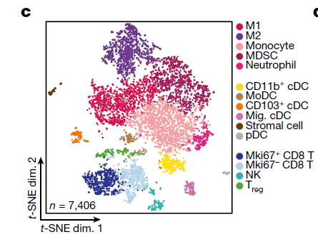
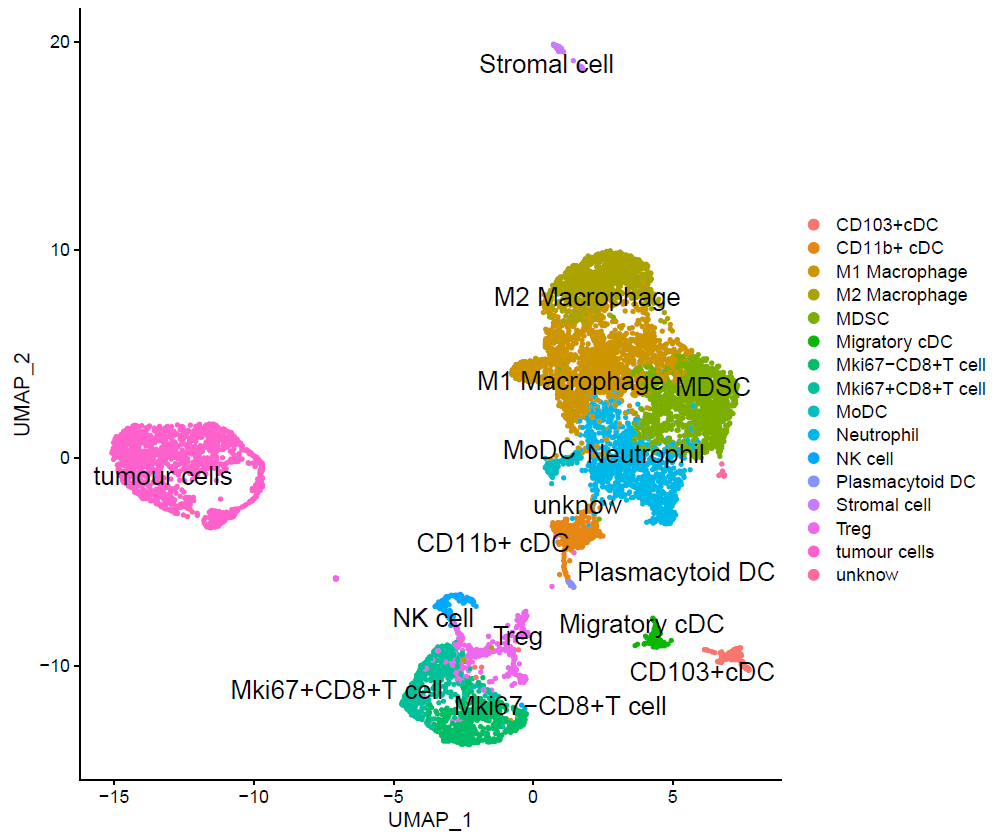
本次研究总共是8000多个单细胞,但是研究者绘制tSNE图的时候,去除了肿瘤细胞,仅仅是展示了7000多个微环境细胞,如下所示:
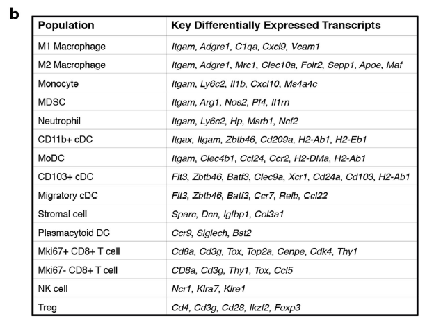
作者在附件列出来了详细的细胞亚群注释依据:
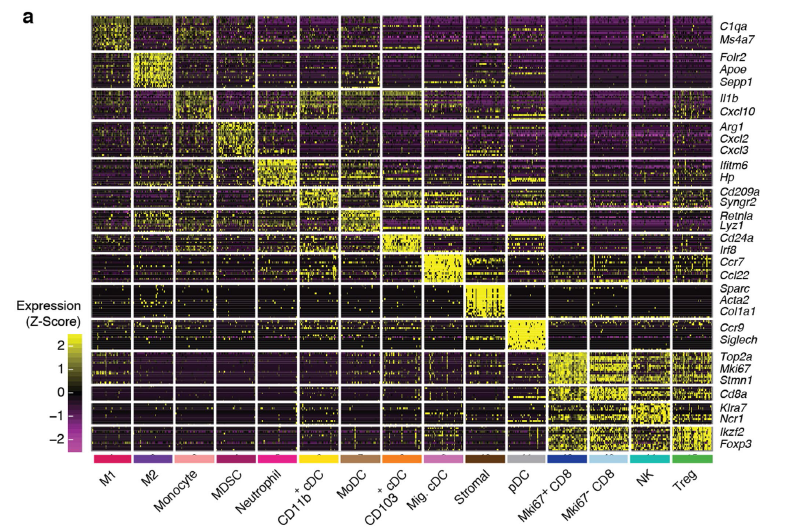
可以看到每个亚群的特异性基因的高表达情况:
开始复现
首先保证 运行环境下面有一个 GSE110746 文件夹,里面有3个文件,如下所示:
$ ls -lh GSE110746
total 295M
-rw-r--r-- 1 win10 197121 230K Feb 17 2018 barcodes.tsv
-rw-r--r-- 1 win10 197121 724K Feb 16 2018 genes.tsv
-rw-r--r-- 1 win10 197121 293M Feb 16 2018 matrix.mtx
数据链接是:https://www.ncbi.nlm.nih.gov/geo/query/acc.cgi?acc=GSE110746
step1构建对象
rm(list=ls())
options(stringsAsFactors = F)
library(tidyverse) # Easily Install and Load the 'Tidyverse'
library(patchwork) # The Composer of Plots
library(Seurat) # Tools for Single Cell Genomics
## 读取数据
scrna_data <- Read10X(data.dir = "GSE110746/")
#构建Seurat对象
seob <- CreateSeuratObject(
 counts = scrna_data, # 表达矩阵可以是稀疏矩阵也可以是普通的矩阵
 min.cells = 3, # 筛选去除小于3个细胞中表达的基因
 min.features = 200) # 去除只有200个一下基因的表达细胞
meat.data <- seob[[]]
dim(seob)
seob[["sample"]] <- gsub(".*-","",rownames(meat.data))
seob = NormalizeData(seob)
dim(seob)
save(seob,file = "201.RData")
step2进行多样品整合
因为是 4个样品:
GSM3015874 Adar_replicate_1
GSM3015875 Adar__replicate_2
GSM3015876 Control_replicate_1
GSM3015877 Control_replicate_2
这里采用 SCT 方法 :
# SCT法整合数据
rm(list=ls())
options(stringsAsFactors = F)
load(file = "201.RData")
# 1. SCTransform
seob_list <- SplitObject(seob, split.by = "sample") # split.by 与52行对应
seob_list
# 查找指定基因
# grep("Mlana",rownames(seob))
# grep("Apoe",rownames(seob))
for(i in 1:length(seob_list)){
 seob_list[[i]] <- SCTransform(
 seob_list[[i]],
 variable.features.n = 3000,
 # vars.to.regress = c("percent.mt", "S.Score", "G2M.Score"),
 verbose = FALSE)
}

# 2. 数据整合(Integration)
## 选择要用于整合的基因
features <- SelectIntegrationFeatures(object.list = seob_list,
 nfeatures = 3000)
## 准备整合
seob_list <- PrepSCTIntegration(object.list = seob_list,
 anchor.features = features)
## 找 anchors,15到30分钟
anchors <- FindIntegrationAnchors(object.list = seob_list,
 # reference = 3 # 当有多个样本时,制定一个作为参考可加快速度
 normalization.method = "SCT", # 选择方法“SCT”
 anchor.features = features
)
## 整合数据
seob <- IntegrateData(anchorset = anchors,
 normalization.method = "SCT")
DefaultAssay(seob) <- "integrated"
save(seob,file = "meta_PCA.RData")
# 我们测试了seurat的V3和V4版本的包,跑这个代码,结果居然是不一样的!
上面的代码以 seurat的V3版本为准,如果是V4,后面的聚类分群数量不一致。
多个样品的整合
这里虽然是选择了SCT,其实CCA也可以,或者说harmony也可以,并没有太大的差异哈!仅仅是一个示例哦
step3 降维聚类分群
## 降维分析----
library(tidyverse) # Easily Install and Load the 'Tidyverse'
library(patchwork) # The Composer of Plots
library(Seurat) # Tools for Single Cell Genomics
load(file = "meta_PCA.RData")
seob <- RunPCA(seob)
ElbowPlot(seob, ndims = 50)
## t-SNE 不是基于表达矩阵做的,而是基于PCA结果做的
seob <- RunTSNE(seob,
 # 使用多少个PC,如果使用的是 SCTransform 建议多一些
 dims = 1:30)

## UMAP
seob <- RunUMAP(seob, dims = 1:30)

# # 检查连续型协变量:线粒体比例
FeaturePlot(seob,
 reduction = "umap", # pca, umap, tsne
 features = "percent.mt")

## 聚类分析 -----
seob <- FindNeighbors(seob,
 k.param = 5,# 最小值为5
 dims = 1:30)
seob <- FindClusters(seob,
 resolution = 0.4, # 分辨率值越大,cluster 越多0~1之间
 random.seed = 1) #设置随机种子
DimPlot(seob,
 reduction = "umap", # pca, umap, tsne
 group.by = "seurat_clusters",
 label = T)
如下所示:
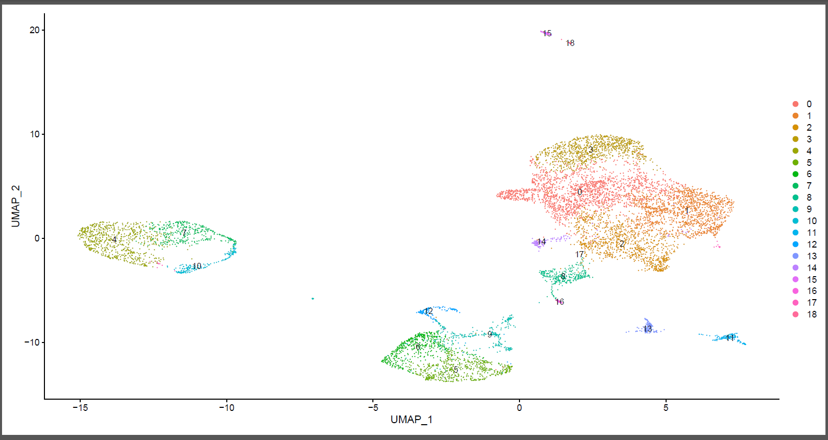
如果是seurat V4 ,同样的代码得到细胞亚群并不一致哦!如果是harmony或者CCA整合,也不一样,感兴趣的可以自行去测试哈!
step4 细胞亚群注释
首先看文章里面的标记基因在各个亚群的表达情况:
library(SummarizedExperiment)
## 构建CellMarker文件
# 这个文件来源于文章,强烈 依赖于生物学背景
library(readr)
cell_marker <- read.table(file = "marker.txt",
 sep = "\t",
 header = T)
cell_marker
## marker 基因表达

## 可视化
library(tidyr)
cell_marker <- separate_rows(cell_marker, Cell_Marker, sep = ",") %>% # 转为长数据
 distinct() %>% # 去除重复
 arrange(Cell_Type) # 排序

p1 <- DimPlot(seob,
 reduction = "umap", # pca, umap, tsne
 group.by = "seurat_clusters",
 label = T)

p2 <- DotPlot(seob, features = unique(cell_marker$Cell_Marker)) +
 theme(axis.text = element_text(size = 8,# 修改基因名的位置
 angle = 45,
 hjust = 1))
p1 + p2
ggsave(plot = p1,filename = 'umap.pdf')

ggsave(plot = p2,filename = 'markers.pdf')

DotPlot(seob,
 features = c("Pmel","Mlana")) +
 theme(axis.text = element_text(size = 8,# 修改基因名的位置
 angle = 45,
 hjust = 1))
如下所示:
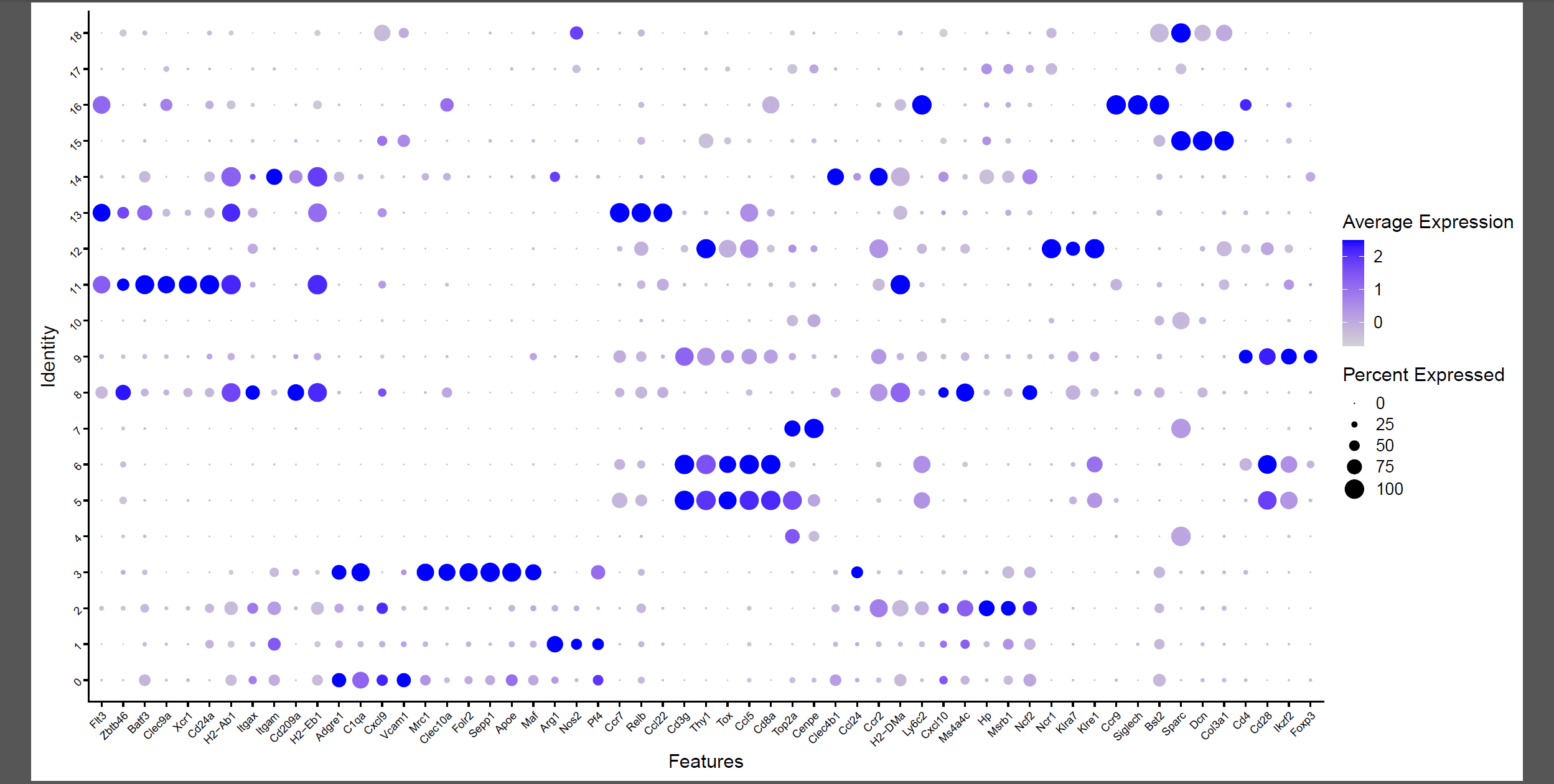
高表达不同基因的亚群可以根据生物学背景进行命名:
## 将细胞类型信息加到meat.data表中
## 构建细胞类型向量

# 这个是肉眼看,依据生物学背景
# 所以每次都需要修改

# 一定要自己肉眼看各个标记基因哦!
# 然后决定下面的分群
# 首先我们看 seurat V4版本的是 0-13的群
grep("ll1b",rownames(seob))
cluster2type <- c("0"="MDSC",
 "1"="M1 Macrophage",
 "2"="tumour cells",
 "3"="Mki67-CD8+T cell",
 "4"="M2 Macrophage",
 "5"="Neutrophil",
 "6"="Mki67+CD8+T cell",
 "7"="Monocyte",
 "8"="tumour cells",
 "9"="CD103+cDC",
 "10"="Migratory cDC",
 "11"="MoDC",
 "12"="Stromal cell",
 "13"="Plasmacytoid")

# 然后看seurat V3版本的是 0-18的群
# Seurat_v3
cluster2type <- c("0"="M1 Macrophage",
 "1"="MDSC",
 "2"="Neutrophil",
 "3"="M2 Macrophage",
 "4"="tumour cells",
 "5"="Mki67-CD8+T cell",
 "6"="Mki67+CD8+T cell",
 "7"="tumour cells",
 "8"="CD11b+ cDC",
 "9"="Treg",
 "10"="tumour cells",
 "11"="CD103+cDC",
 "12"="NK cell",
 "13"="Migratory cDC",
 "14"="MoDC",
 "15"="Stromal cell",
 "16"="Plasmacytoid DC",
 "17"="", #未找到高变基因
 "18"="Stromal cell")

## 可视化
## 二维图
FeaturePlot(seob,
 reduction = "umap",
 features = c("Pmel","Mlana"),
 #split.by = "sample",
 label = TRUE)

## 小提琴图
VlnPlot(object = seob,
 features = c("Pmel","Mlana")) + plot_layout(guides = "collect") & theme(legend.position = "top")

## 添加细胞类型

seob[['cell_type']] = unname(cluster2type[seob@meta.data$seurat_clusters])

DimPlot(seob,
 reduction = "umap",
 group.by = "cell_type",
 label = TRUE, pt.size = 1,
 label.size = 6,
 repel = TRUE)
最后拿到了有生物学意义的亚群:
这就是完成了最基础的聚类分群和注释,也可以参考其它例子,比如:人人都能学会的单细胞聚类分群注释
如果你没有单细胞转录组数据分析的基础知识,可以先一下基础10讲: