去年我们在《生信技能树》公众号带领大家一起学习过:[SCENIC转录因子分析结果的解读](https://mp.weixin.qq.com/s/eAfkhX0SJu1lytZeXdsh0Q) ,提到了在做单细胞转录因子分析,首选的工具就是SCENIC流程,其工作流程两次发表在nature系列杂志足以说明它的优秀 :
- SCENIC : single-cell regulatory network inference and clustering(2017年的nature methods)
- A scalable SCENIC workflow for single-cell gene regulatory network analysis(2020年的nature protocls)
SCENIC (Single-Cell rEgulatory Network Inference and Clustering) is a computational method to infer Gene Regulatory Networks and cell types from single-cell RNA-seq data. 官网教程非常清晰:
提供了 (R / Python)两个版本的运行方式 ,SCENIC is implemented in R (this package and tutorial) and Python (pySCENIC).
安装SCENIC流程
其中R语言版本的SCENIC流程依赖于3个R包:
- GENIE3 to infer the co-expression network (faster alternative: GRNBoost2)
- RcisTarget for the analysis of transcription factor binding motifs
- AUCell to identify cells with active gene sets (gene-network) in scRNA-seq data
所以,实际上学习这个SCENIC流程,必须要先学习这3个R包的。
比如RcisTarget 包,基于DNA-motif 分析选择潜在的直接结合靶点,我也是写了两个教程:
再比如那个AUCell 包,我分享了:使用AUCell包的AUCell_calcAUC函数计算每个细胞的每个基因集的活性程度
安装它们的话基本上复制粘贴下面的代码即可:
if (!requireNamespace("BiocManager", quietly = TRUE)) install.packages("BiocManager")
BiocManager::version()
# If your bioconductor version is previous to 4.0, see the section bellow

## Required
BiocManager::install(c("AUCell", "RcisTarget"),ask = F,update = F)
BiocManager::install(c("GENIE3"),ask = F,update = F) # Optional. Can be replaced by GRNBoost

## Optional (but highly recommended):
# To score the network on cells (i.e. run AUCell):
BiocManager::install(c("zoo", "mixtools", "rbokeh"),ask = F,update = F)
# For various visualizations and perform t-SNEs:
BiocManager::install(c("DT", "NMF", "ComplexHeatmap", "R2HTML", "Rtsne"),ask = F,update = F)
# To support paralell execution (not available in Windows):
BiocManager::install(c("doMC", "doRNG"),ask = F,update = F)
# To export/visualize in http://scope.aertslab.org
if (!requireNamespace("devtools", quietly = TRUE)) install.packages("devtools")
devtools::install_github("aertslab/SCopeLoomR", build_vignettes = TRUE)

if (!requireNamespace("devtools", quietly = TRUE)) install.packages("devtools")
devtools::install_github("aertslab/SCENIC")
packageVersion("SCENIC")
Python我不怎么使用,所以 Python (pySCENIC). 先略过。虽然这次略过了,但其实是躲不过去的,因为R里面的计算速度真心很慢,后期我们会补上这个 Python (pySCENIC). 教程哈。
另外,运行单细胞转录因子分析之SCENIC流程还需要下载配套数据库,不同物种不一样, 在 https://resources.aertslab.org/cistarget/ 查看自己的物种,按需下载:
# https://resources.aertslab.org/cistarget/
dbFiles <- c("https://resources.aertslab.org/cistarget/databases/homo_sapiens/hg19/refseq_r45/mc9nr/gene_based/hg19-500bp-upstream-7species.mc9nr.feather",
 "https://resources.aertslab.org/cistarget/databases/homo_sapiens/hg19/refseq_r45/mc9nr/gene_based/hg19-tss-centered-10kb-7species.mc9nr.feather")
# dir.create("cisTarget_databases"); setwd("cisTarget_databases") # if needed
dbFiles <- c("https://resources.aertslab.org/cistarget/databases/mus_musculus/mm9/refseq_r45/mc9nr/gene_based/mm9-500bp-upstream-7species.mc9nr.feather",
 "https://resources.aertslab.org/cistarget/databases/mus_musculus/mm9/refseq_r45/mc9nr/gene_based/mm9-tss-centered-10kb-7species.mc9nr.feather")
# mc9nr: Motif collection version 9: 24k motifs
dbFiles
for(featherURL in dbFiles)
{
 download.file(featherURL, destfile=basename(featherURL)) # saved in current dir
 # (1041.7 MB)
 #
}
每个文件都是1G,下载好了存放在共享文件夹,可以多台电脑传输使用,没有必要每次都下载。而且可以看到,参考基因组版本并不是最新哦,人类的话这里使用hg19,小鼠使用mm9,都是很久以前的参考基因组啦。
SCENIC分析流程
下面才进入正餐!
输入数据的准备:表达矩阵加上表型信息
跟 CellPhoneDB运行需要的输入数据一样,也是表达矩阵加上表型信息即可,官网给出的示例数据是基于loom文件,实际上没有这个必要哈,最重要的是 表达矩阵加上表型信息 :
rm(list = ls())
library(SCENIC)

## Load data
loomPath <- system.file(package="SCENIC", "examples/mouseBrain_toy.loom")
library(SCopeLoomR)
loom <- open_loom(loomPath)
exprMat <- get_dgem(loom)
cellInfo <- get_cell_annotation(loom)
close_loom(loom)

dim(exprMat)
exprMat[1:4,1:4]
head(cellInfo)
table(cellInfo$CellType)
可以看到是,这个官方例子是从loom文件里面提取的小鼠的表达矩阵,200个细胞分成5个亚群,基因数量就862个。这个数据量可以说是非常小啦,所以运行这个流程会很快哈。
> dim(exprMat)
[1] 862 200
> exprMat[1:4,1:4]
 1772066100_D04 1772063062_G01 1772060224_F07 1772071035_G09
Arhgap18 0 0 0 0
Apln 0 0 0 0
Cnn3 0 0 0 0
Eya1 0 0 0 4
> head(cellInfo)
 CellType nGene nUMI
1772066100_D04 interneurons 170 509
1772063062_G01 oligodendrocytes 152 443
1772060224_F07 microglia 218 737
1772071035_G09 pyramidal CA1 265 1068
1772067066_E12 oligodendrocytes 81 273
1772066100_B01 pyramidal CA1 108 191
> table(cellInfo$CellType)

astrocytes_ependymal interneurons microglia oligodendrocytes pyramidal CA1
 29 43 14 55 59
>
但是呢,我们自己的数据一般是在Seurat的对象里面,很容易制作这样的的两个信息:表达矩阵加上表型信息。后面我也有一个示例来讲解。
数据库文件的准备
不同物种不一样, 在 https://resources.aertslab.org/cistarget/ 查看自己的物种,按需下载,因为示例数据是小鼠表达矩阵,所以这里我们下载小鼠的,并且构建了一个 cisTarget_databases 文件夹 来存放下载好的数据库文件。
### Initialize settings
library(SCENIC)
# 保证 cisTarget_databases 文件夹下面有下载好2个1G的文件
scenicOptions <- initializeScenic(org="mgi", dbDir="cisTarget_databases", nCores=10)
# scenicOptions@inputDatasetInfo$cellInfo <- "int/cellInfo.Rds"
saveRDS(scenicOptions, file="int/scenicOptions.Rds")
需要注意的是,nCores=10 在部分电脑上面不适用哦,主要是没办法开启并行计算。会报错如下:
Using 10 cores.
Warning in .AUCell_calcAUC(geneSets = geneSets, rankings = rankings, nCores = nCores, :
 Using only the first 58.99 genes (aucMaxRank) to calculate the AUC.
Error in .AUCell_calcAUC(geneSets = geneSets, rankings = rankings, nCores = nCores, :
 Valid 'mctype': 'snow' or 'doMC'
解决方案是修改代码为 nCores=1 即可。
这个时候,该流程会自动新建两个文件夹,一个是 int文件夹,一个是output文件夹。
运行SCENIC流程
首先是最耗费时间的步骤,Co-expression network
因为这个示例数据是小鼠表达矩阵200个细胞分成5个亚群,基因数量就862个。这个数据量可以说是非常小啦,所以运行这个流程会很快哈。但是实际情况下,这个步骤至少耗费几个小时,甚至好几天,建议挂在后台慢慢运行。
### Co-expression network
genesKept <- geneFiltering(exprMat, scenicOptions)
exprMat_filtered <- exprMat[genesKept, ]
exprMat_filtered[1:4,1:4]
runCorrelation(exprMat_filtered, scenicOptions)
exprMat_filtered_log <- log2(exprMat_filtered+1)
runGenie3(exprMat_filtered_log, scenicOptions)
可以看到,我们的小鼠表达矩阵200个细胞分成5个亚群,基因数量就862个,这里面呢,属于转录因子的居然仅仅是8个基因,所以函数会提醒一下: Only 8 (0%) of the 1721 TFs in the database were found in the dataset. Do they use the same gene IDs?
其中这个 runGenie3 流程是限速步骤,可以转移到服务器上面运行,或者走对应的 Python (pySCENIC). 版本。
然后是SCENIC流程的4个步骤
SCENIC流程其实是包装好的4个函数,有了前面的数据和数据库挖掘,完成起来非常快,如下:
runSCENIC_1_coexNetwork2modules(scenicOptions)
runSCENIC_2_createRegulons(scenicOptions, coexMethod=c("top5perTarget")) # Toy run settings
runSCENIC_3_scoreCells(scenicOptions, exprMat_log)
runSCENIC_4_aucell_binarize(scenicOptions)
这4个函数分别完成下面的4个分析环节:
- GENIE3/GRNBoost:基于共表达情况鉴定每个TF的潜在靶点;
- RcisTarget:基于DNA-motif 分析选择潜在的直接结合靶点;
- AUCell:分析每个细胞的regulons活性;
- 细胞聚类:基于regulons的活性鉴定稳定的细胞状态并对结果进行探索
前面的3个步骤依次使用一个R包,所以原则上需要独立去学习每个R包的用法。 大家千万不要妄想就看几次教程就学会了,一定要亲自实践。代码如下:
### Build and score the GRN
exprMat_log <- log2(exprMat+1)
scenicOptions@settings$dbs <- scenicOptions@settings$dbs["10kb"] # Toy run settings
scenicOptions <- runSCENIC_1_coexNetwork2modules(scenicOptions)
scenicOptions <- runSCENIC_2_createRegulons(scenicOptions, coexMethod=c("top5perTarget")) # Toy run settings
scenicOptions <- runSCENIC_3_scoreCells(scenicOptions, exprMat_log)

scenicOptions <- runSCENIC_4_aucell_binarize(scenicOptions)
tsneAUC(scenicOptions, aucType="AUC") # choose settings
运行的log日志是:
> scenicOptions <- runSCENIC_1_coexNetwork2modules(scenicOptions)
17:23 Creating TF modules
Number of links between TFs and targets (weight>=0.001): 6139
 [,1]
nTFs 8
nTargets 770
nGeneSets 47
nLinks 17299
> scenicOptions <- runSCENIC_2_createRegulons(scenicOptions, coexMethod=c("top5perTarget")) # Toy run settings
17:23 Step 2. Identifying regulons
tfModulesSummary:
 [,1]
top5perTarget 8
17:23 RcisTarget: Calculating AUC
Scoring database: [Source file: mm9-tss-centered-10kb-7species.mc9nr.feather]
17:23 RcisTarget: Adding motif annotation
Using BiocParallel...
Number of motifs in the initial enrichment: 867
Number of motifs annotated to the matching TF: 126
17:23 RcisTarget: Prunning targets
17:24 Number of motifs that support the regulons: 126
 Preview of motif enrichment saved as: output/Step2_MotifEnrichment_preview.html
Warning messages:
1: In RcisTarget::importRankings(dbFilePath, columns = randomCol) :
 The following columns are missing from the database:
2: In importRankings(rnkName, columns = allGenes) :
 The following columns are missing from the database:
3: In importRankings(dbNames[motifDbName], columns = allGenes) :
 The following columns are missing from the database:
4: In .addSignificantGenes(resultsTable = resultsTable, geneSets = geneSets, :
 The rakings provided only include a subset of genes/regions included in the whole database.
> scenicOptions <- runSCENIC_3_scoreCells(scenicOptions, exprMat_log)
17:24 Step 3. Analyzing the network activity in each individual cell
 Number of regulons to evaluate on cells: 14
Biggest (non-extended) regulons:
 Tef (405g)
 Sox9 (150g)
 Irf1 (104g)
 Sox8 (97g)
 Sox10 (88g)
 Dlx5 (35g)
 Stat6 (27g)
Quantiles for the number of genes detected by cell:
(Non-detected genes are shuffled at the end of the ranking. Keep it in mind when choosing the threshold for calculating the AUC).
 min 1% 5% 10% 50% 100%
 46.00 58.99 77.00 84.80 154.00 342.00
Warning in .AUCell_calcAUC(geneSets = geneSets, rankings = rankings, nCores = nCores, :
 Using only the first 58.99 genes (aucMaxRank) to calculate the AUC.
17:24 Finished running AUCell.
17:24 Plotting heatmap...
17:24 Plotting t-SNEs...
> scenicOptions <- runSCENIC_4_aucell_binarize(scenicOptions)
Binary regulon activity: 7 TF regulons x 200 cells.
(13 regulons including 'extended' versions)
7 regulons are active in more than 1% (2) cells.

> scenicOptions <- runSCENIC_4_aucell_binarize(scenicOptions)
Binary regulon activity: 7 TF regulons x 200 cells.
(13 regulons including 'extended' versions)
7 regulons are active in more than 1% (2) cells.
> tsneAUC(scenicOptions, aucType="AUC") # choose settings
[1] "int/tSNE_AUC_50pcs_30perpl.Rds"
到此为止,全部的SCENIC流程运行完毕,输出数据都是在output文件夹,剩下来的就是解读它了。不过,因为是测试数据,小鼠的表达矩阵,200个细胞分成5个亚群,基因数量就862个。所以这个结果解读的意义也不大,我们还是直接来一个实战吧!
实战(以Seurat的pbmc3K数据集为例)
下面的代码复制粘贴即可运行,超级简单,如果是你自己的数据,你只需同样的模式做出来 exprMat 表达矩阵,和cellInfo的临床表型,就可以走这个SCENIC流程的4个步骤啦。
rm(list = ls())
library(Seurat)
# devtools::install_github('satijalab/seurat-data')
library(SeuratData)
AvailableData()
# InstallData("pbmc3k") # (89.4 MB)
data("pbmc3k")
exprMat <- as.matrix(pbmc3k@assays$RNA@data)
dim(exprMat)
exprMat[1:4,1:4]
cellInfo <- pbmc3k@meta.data[,c(4,2,3)]
colnames(cellInfo)=c('CellType', 'nGene' ,'nUMI')
head(cellInfo)
table(cellInfo$CellType)

### Initialize settings
library(SCENIC)
# 保证cisTarget_databases 文件夹下面有下载好2个1G的文件
scenicOptions <- initializeScenic(org="hgnc",
 dbDir="cisTarget_databases", nCores=1)
saveRDS(scenicOptions, file="int/scenicOptions.Rds")

### Co-expression network
genesKept <- geneFiltering(exprMat, scenicOptions)
exprMat_filtered <- exprMat[genesKept, ]
exprMat_filtered[1:4,1:4]
dim(exprMat_filtered)
runCorrelation(exprMat_filtered, scenicOptions)
exprMat_filtered_log <- log2(exprMat_filtered+1)
runGenie3(exprMat_filtered_log, scenicOptions)

### Build and score the GRN
exprMat_log <- log2(exprMat+1)
scenicOptions@settings$dbs <- scenicOptions@settings$dbs["10kb"] # Toy run settings
scenicOptions <- runSCENIC_1_coexNetwork2modules(scenicOptions)
scenicOptions <- runSCENIC_2_createRegulons(scenicOptions,
 coexMethod=c("top5perTarget")) # Toy run settings
library(doParallel)
scenicOptions <- runSCENIC_3_scoreCells(scenicOptions, exprMat_log )
scenicOptions <- runSCENIC_4_aucell_binarize(scenicOptions)
tsneAUC(scenicOptions, aucType="AUC") # choose settings
上面代码就完成了!
因为我们这个是实战案例,表达矩阵很大,接近3000个细胞,是全部的人类基因,所以耗费了一个晚上才完成这个流程,运行的log日志如下:
> runGenie3(exprMat_filtered_log, scenicOptions)
Using 480 TFs as potential regulators...
Running GENIE3 part 1
Running GENIE3 part 10
Running GENIE3 part 2
Running GENIE3 part 3
Running GENIE3 part 4
Running GENIE3 part 5
Running GENIE3 part 6
Running GENIE3 part 7
Running GENIE3 part 8
Running GENIE3 part 9
Finished running GENIE3.
>
> ### Build and score the GRN
> exprMat_log <- log2(exprMat+1)
> scenicOptions@settings$dbs <- scenicOptions@settings$dbs["10kb"] # Toy run settings
> scenicOptions <- runSCENIC_1_coexNetwork2modules(scenicOptions)
07:33 Creating TF modules
Number of links between TFs and targets (weight>=0.001): 1773984
 [,1]
nTFs 480
nTargets 5318
nGeneSets 3835
nLinks 2516422
> scenicOptions <- runSCENIC_2_createRegulons(scenicOptions,
+ coexMethod=c("top5perTarget")) # Toy run settings
07:34 Step 2. Identifying regulons
tfModulesSummary:
 [,1]
top5perTarget 59
07:34 RcisTarget: Calculating AUC
Scoring database: [Source file: hg19-tss-centered-10kb-7species.mc9nr.feather]
07:35 RcisTarget: Adding motif annotation
Using BiocParallel...
Number of motifs in the initial enrichment: 18696
Number of motifs annotated to the matching TF: 334
07:35 RcisTarget: Prunning targets
07:37 Number of motifs that support the regulons: 334
 Preview of motif enrichment saved as: output/Step2_MotifEnrichment_preview.html
> library(doParallel)
Loading required package: iterators
> scenicOptions <- runSCENIC_3_scoreCells(scenicOptions, exprMat_log )
07:37 Step 3. Analyzing the network activity in each individual cell
 Number of regulons to evaluate on cells: 20
Biggest (non-extended) regulons:
 SPI1 (538g)
 CEBPB (47g)
 CEBPD (41g)
 SPIB (39g)
 TBX21 (27g)
 IRF8 (17g)
 STAT1 (14g)
 IRF7 (12g)
Quantiles for the number of genes detected by cell:
(Non-detected genes are shuffled at the end of the ranking. Keep it in mind when choosing the threshold for calculating the AUC).
 min 1% 5% 10% 50% 100%
 212.00 325.00 434.95 539.90 816.00 3400.00
07:38 Finished running AUCell.
07:38 Plotting heatmap...
07:38 Plotting t-SNEs...
> scenicOptions <- runSCENIC_4_aucell_binarize(scenicOptions)
Binary regulon activity: 11 TF regulons x 1678 cells.
(19 regulons including 'extended' versions)
11 regulons are active in more than 1% (16.78) cells.
> tsneAUC(scenicOptions, aucType="AUC") # choose settings
[1] "int/tSNE_AUC_50pcs_30perpl.Rds"
可以看到,对于我们这个真实数据,就是PBMC3K的,也只有19个regulon被挑选出来了,涉及到11个TF基因
作者推荐的运算结果保存是:
export2loom(scenicOptions, exprMat)
saveRDS(scenicOptions, file="int/scenicOptions.Rds")
实际上我们也用不上哈!
输出结果的解读
首先看看转录因子富集结果:
rm(list = ls())
library(Seurat)
library(SCENIC)
library(doParallel)

scenicOptions=readRDS(file="int/scenicOptions.Rds")

### Exploring output
# Check files in folder 'output'
# Browse the output .loom file @ http://scope.aertslab.org

# output/Step2_MotifEnrichment_preview.html in detail/subset:
motifEnrichment_selfMotifs_wGenes <- loadInt(scenicOptions, "motifEnrichment_selfMotifs_wGenes")
as.data.frame(sort(table(motifEnrichment_selfMotifs_wGenes$highlightedTFs),decreasing = T))
每个基因的motif数量:
> as.data.frame(sort(table(motifEnrichment_selfMotifs_wGenes$highlightedTFs),decreasing = T))
 Var1 Freq
1 SPI1 61
2 IRF7 59
3 TBX21 47
4 STAT1 33
5 SPIB 27
6 MAFB 26
7 IRF8 23
8 CEBPD 21
9 FOS 10
10 POU2AF1 5
11 CEBPB 3
12 TCF7 3
13 MAX 2
14 FOSB 1
15 LEF1 1
16 LYL1 1
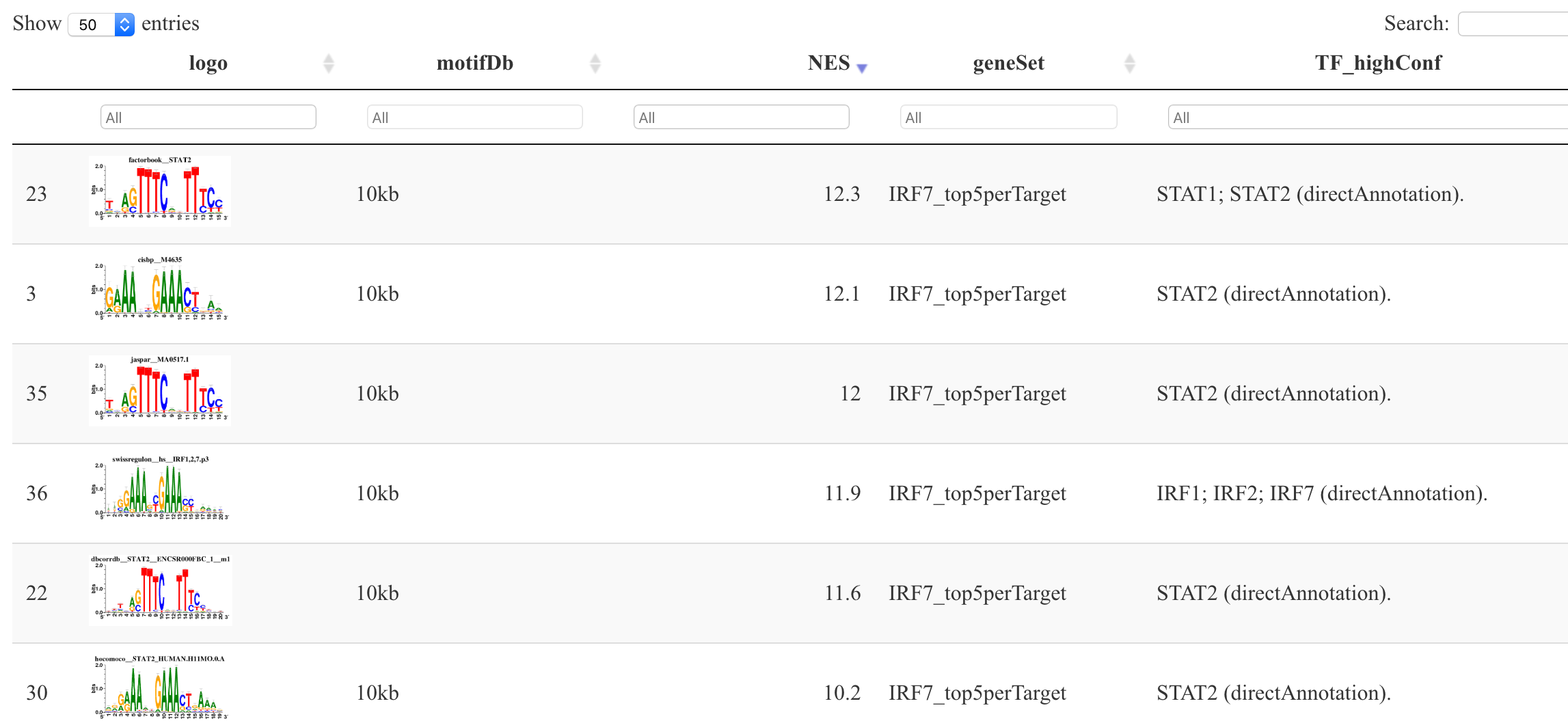
可视化IRF7基因的motif序列特征:
tableSubset <- motifEnrichment_selfMotifs_wGenes[highlightedTFs=="IRF7"]
viewMotifs(tableSubset)
这个时候的IRF7基因有 56 个motif,如下所示:
如果加上活性单元(regulon)的限定后:
regulonTargetsInfo <- loadInt(scenicOptions, "regulonTargetsInfo")
tableSubset <- regulonTargetsInfo[TF=="IRF7" & highConfAnnot==TRUE]
viewMotifs(tableSubset)
就只有12个啦,不过我们需要的并不是这些结果啦。
如果要理解(regulon),需要看我分享的:使用AUCell包的AUCell_calcAUC函数计算每个细胞的每个基因集的活性程度
可以使用的结果:
其中output文件夹本来就已经自动绘制了大量的图表供使用,而图表对应的数据就存储在 loomFile 里面,可以使用下面的代码重新获取:
rm(list = ls())
library(Seurat)
library(SCENIC)
library(doParallel)
library(SCopeLoomR)
scenicOptions=readRDS(file="int/scenicOptions.Rds")
scenicLoomPath <- getOutName(scenicOptions, "loomFile")
loom <- open_loom(scenicLoomPath)
# Read information from loom file:
regulons_incidMat <- get_regulons(loom)
regulons <- regulonsToGeneLists(regulons_incidMat)
regulonsAUC <- get_regulons_AUC(loom)
regulonsAucThresholds <- get_regulon_thresholds(loom)
embeddings <- get_embeddings(loom)
可以可视化其中一些TF的AUC值,也可以根据这些TF的AUC值对细胞亚群进行重新降维聚类分群。可以很容易看到血液里面的不同细胞亚群的特异性的转录调控因子:
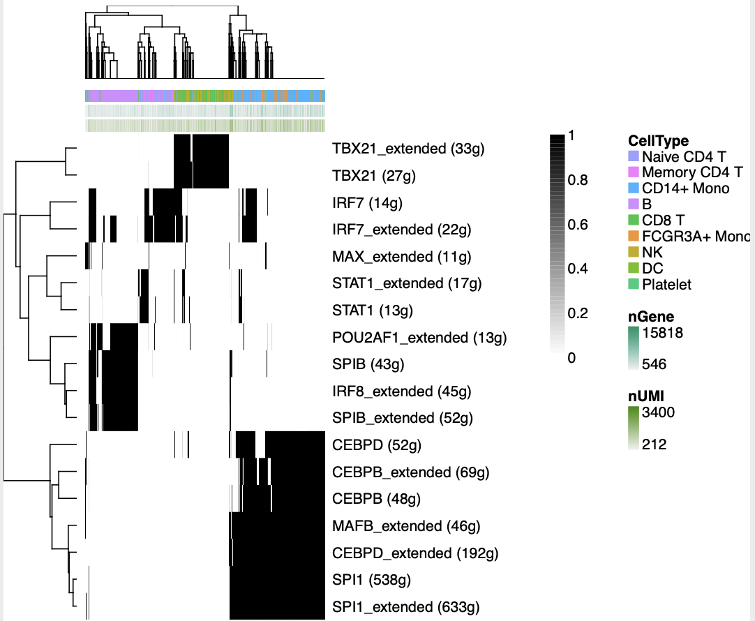
如果使用这些转录调控因子进行 降维聚类分群 ,可以得到:

更多文章实例图表可以看:SCENIC转录因子分析结果的解读 ,这里面我埋下了两个伏笔,都是关于R里面的这个单细胞转录因子分析之SCENIC流程运行超级慢的问题,仅仅是接近3000个细胞就耗费了一个晚上才完成这个流程,现在的单细胞研究,动辄是几万个细胞,这个流程要是搞几个星期就不得了了。我后面会继续讲解关于这个问题的两个解决方案,第一个是对细胞亚群里面的单细胞进行抽样,第二个是 Python (pySCENIC). 教程,开启多线程!