又是老板扔来得一篇单细胞数据的文章!话不多说,撸起袖子加油干~
值得注意的是,我目前的水平只能是做到单细胞转录组数据的预处理,降维聚类分群。高阶分析还没有学到,不过隔壁《单细胞天地》有一个活动,感兴趣的可以参加一下:单细胞进阶数据分析技巧一网打尽,名额有限,大家赶快抢哈!
文章信息如下:
标题:Single cell analysis of the normal mouse aorta reveals functionally distinct endothelial cell populations
Published :Circulation. 2019 July 09; 140(2): 147–163. doi:10.1161/CIRCULATIONAHA.118.038362
1.数据下载
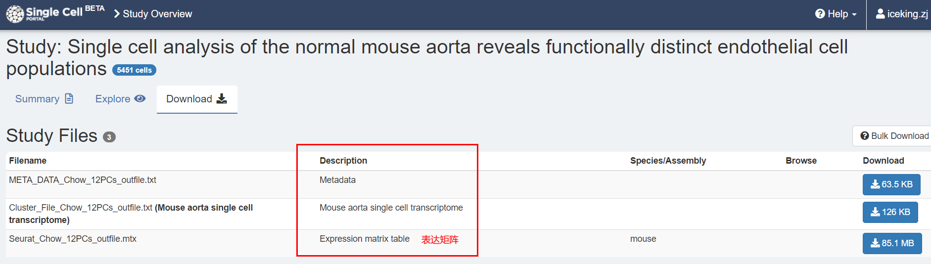
阅读原文,找到提供得数据:
The raw counts table and the normalized expression table for the high-depth normal mouse
aorta transcriptional profile are publicly available via the Broad Institute Single Cell Portal:
https://portals.broadinstitute.org/single_cell/study/SCP289/single-cell-analysis-of-thenormal-mouse-aorta-reveals-functionally-distinct-endothelial-cell-populations.
2.走单细胞标准流程
文章中给出的各种细节:
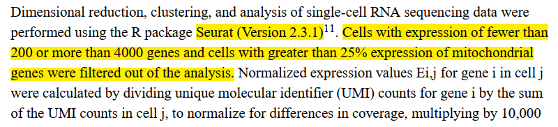
过滤指标:
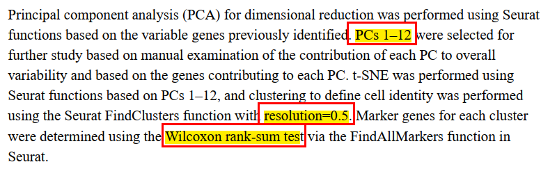
其他参数选择:
代码如下:
rm(list=ls())
options(stringsAsFactors = F)

library(Seurat)
library(ggplot2)
counts <- read.table("../data/Seurat_Chow_12PCs_outfile.mtx",header = T,sep="",check.names = F,row.names=1)
counts[1:4,1:4]
dim(counts) # 9260个基因,5451个细胞
总共得到5451个细胞,9k多个基因,而文章中提到的是The high-sequencing depth data was used for all subsequent analyses, and yielded approximately 6,200 cells and 1,900 genes/ cell (Figure 1) ,即6200个细胞,所以我们能够拿到的是处理过后的表达谱了。
还有一点,文章总共测了4个样本,两个low-sequencing depth 以及两个high-sequencing depth ,就提了一句测序深度对聚类细胞数没有影响,后续所有分析都是基于high-sequencing depth得到的数据进行分析的。
啊,既然没有影响,那为什么四个样本不都用呢?
# 临床信息,也只有作者分组得到的类别而已
anno <- read.table("../data/META_DATA_Chow_12PCs_outfile",header = T,sep="\t")
rownames(anno) <- anno$NAME
head(anno)
 NAME Cluster Sub.Cluster Average.Intensity
TYPE TYPE group group numeric
AAACCTGAGACGCTTT-1 AAACCTGAGACGCTTT-1 VSMC VSMC -1.316880e-02
AAACCTGCACTGTGTA-1 AAACCTGCACTGTGTA-1 VSMC VSMC 7.831023e-02
AAACGGGCACGGATAG-1 AAACGGGCACGGATAG-1 VSMC VSMC -3.950555e-02
AAACGGGGTGTTCTTT-1 AAACGGGGTGTTCTTT-1 VSMC VSMC -5.717870e-02
AAAGATGAGGCTCATT-1 AAAGATGAGGCTCATT-1 VSMC VSMC 1.115755e-02

table(anno$Cluster)
 EC Fibro group Macro Mono Neuron VSMC
 748 1781 1 167 552 44 2159

table(anno$Sub.Cluster)
 EC 1 EC 2 EC 3 Fibro 1 Fibro 2 group Macro Mono 1 Mono 2 Neuron VSMC
 425 229 94 1147 634 1 167 443 109 44 2159
接下来是标准流程
## 2.创建the Seurat对象
endo <- CreateSeuratObject(counts = counts, project = "endo",min.cells = 3, min.features = 200)
endo

endo <- AddMetaData(object = endo, metadata = anno)

grep("^MT-",rownames(endo),value = T) #没有线粒体基因,因为表达谱是作者提供的处理后的
endo[["percent.mt"]] <- PercentageFeatureSet(endo, pattern = "^MT-")

# 绘制特征图
p <- VlnPlot(endo, features = c("nFeature_RNA", "nCount_RNA","percent.mt"), ncol = 3,pt.size = 0)
p
ggsave(filename="../Figure2A.qc.pdf",plot=p,width = 6,height = 5)

## 3.数据标准化
endo <- NormalizeData(endo, normalization.method = "LogNormalize", scale.factor = 10000)
endo <- FindVariableFeatures(endo, selection.method = "vst", nfeatures = 2000)
endo <- ScaleData(endo)

top10 <- head(VariableFeatures(endo), 10)
top10

plot1 <- VariableFeaturePlot(endo,pt.size = 1.2)
plot2 <- LabelPoints(plot = plot1, points = top10, repel = TRUE)
plot2
ggsave(filename="../Figure2C.Features.pdf",plot=plot2,width = 8,height = 8)

## 4.线性降维
endo <- RunPCA(endo, features = VariableFeatures(object = endo),seed.use = NULL)
DimPlot(endo, reduction = "pca",pt.size = 1.2)

endo <- JackStraw(endo, num.replicate = 100)
endo <- ScoreJackStraw(endo, dims = 1:20)

p1 <- JackStrawPlot(endo, dims = 1:20,)
p2 <- ElbowPlot(endo,ndims = 20)
p1+p2 +theme(legend.position="bottom")
ggsave(filename="../Figure2E.pca.pdf",width = 14,height = 8)

## 5.聚类,按照文章中的参数pc=12,resolution=0.5
endo <- FindNeighbors(endo, dims = 1:12)
endo <- FindClusters(endo, resolution = 0.5)

endo <- RunTSNE(endo, dims = 1:12,seed.use = NULL)
p <- DimPlot(endo, reduction = "tsne",pt.size = 1,label = T,label.size = 5)
p
ggsave(filename = "../Figure2F.TSNE.pdf",plot=p,width = 9,height = 8)

## 6.差异表达分析
# find markers for every cluster compared to all remaining cells, report only the positive ones
library(rlang)
library(dplyr)
endo.markers <- FindAllMarkers(endo, only.pos = TRUE, min.pct = 0.25, logfc.threshold = 0.25)
save(endo.markers,file = "../data/endo.markers.RData")
endo.markers %>% group_by(cluster) %>% top_n(n = 2, wt = avg_logFC)

top10 <- endo.markers %>% group_by(cluster) %>% top_n(n = 10, wt = avg_logFC)
p <- DoHeatmap(endo, features = top10$gene,size = 4) + NoLegend() + theme(axis.text.y=element_text(size=5))
ggsave(filename="../Figure2G.DoHeatmap.pdf",plot=p,width = 9,height = 7)
接下来是细胞注释,作者采用的经典markers进行的手动注释,marker列表为附表1,如下:

手动注释过程如下:
## 6.s根据经典markers鉴定细胞类型
Fibroblasts <- c("Pdgfra")
VSMC <- c("Cnn1","Myh11")
EC <- c("Cdh5")
Monocytes <- c("Cd68", "Csf1r", "Lyz2") #Csf1r(Cd115)
T_B_cells <- c("Cd3d", "Cd19")
Macrophage_DC <- c("H2-Ab1", "Cd68")
RBC <- c("Hbb")

all_markers <- c("Pdgfra","Cnn1","Myh11","Cdh5","Cd68","Csf1r","Lyz2","Cd3d","Cd19","H2-Ab1","Hbb")
VlnPlot(endo, features = all_markers,pt.size = 0)
p <- DotPlot(endo, features = all_markers) + coord_flip()
ggsave(filename="../Figure2G.gene2check.pdf",plot=p,width = 9,height = 7)

根据这些指标,注释信息如下:
endo <- RenameIdents(endo,
 `0` = "VSMC",
 `1` = "Fibroblasts",
 `2` = "VSMC",
 `3` = "Fibroblasts",
 `4` = "Monocytes",
 `5` = "EC",
 `6` = "EC",
 `7` = "Macrophage/DC ",
 `8` = "Macrophage/DC",
 `9` = "EC",
 `10` = "Monocytes")

p <- DimPlot(endo, label = TRUE,pt.size = 1.2)
ggsave(filename="../Figure2G.anno.pdf",plot=p,width = 9,height = 7)

与原文相比,还是差了一点点的,哎。
接着,使用文章中的Figure1来进行检查,不知道这个Neuron是怎么出来的啊,marker列表中没有。。。
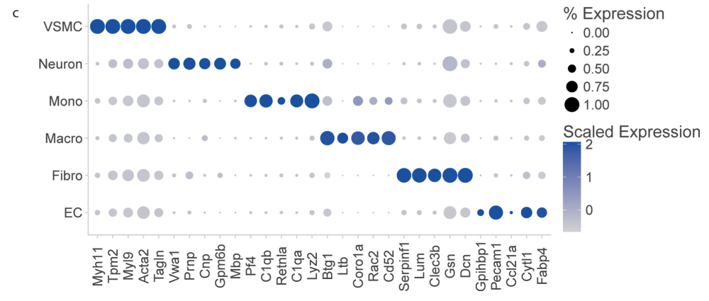
gene2check <- c("Myh11","Tpm2","Myl9","Acta2","Tagln",
 "Vwa1","Prnp","Cnp","Gpm6b","Mbp",
 "Pf4","C1qb","Retnla","C1qa","Lyz2",
 "Btg1","Ltb","Coro1a","Rac2","Cd52",
 "Serpinf1","Lum","Clec3b","Gsn","Dcn",
 "Gpihbp1","Pecam1","Ccl21a","Cytl1","Fabp4")
p <- DotPlot(endo, features = gene2check) + theme(axis.text.x = element_text(angle = 90, hjust = 1))
p
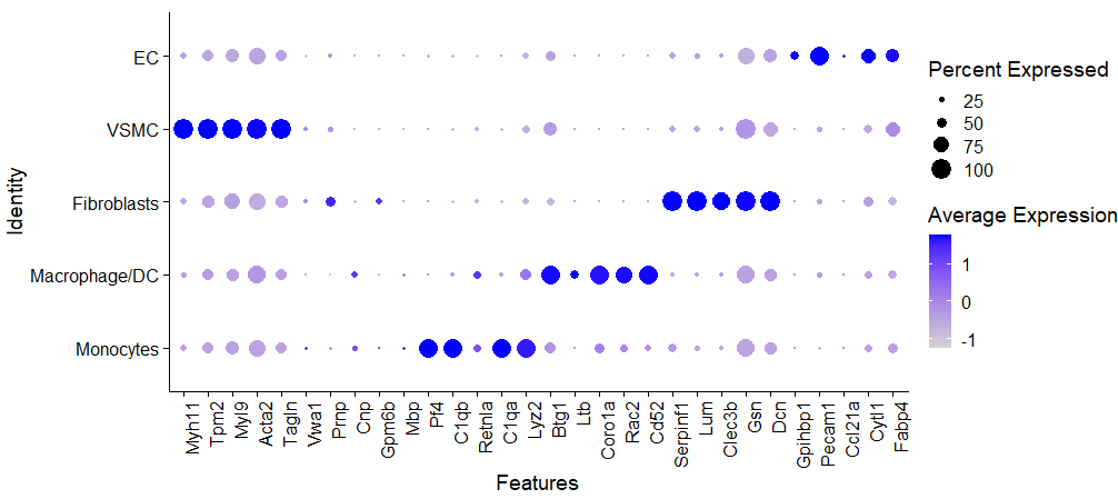
除了突然出现的Neuron,其他基本上都能对上啦。
上面的分析仅仅是转录组表达矩阵的聚类分群,析相信大家都已经掌握的不错了,在《单细胞天地》的单细胞基础10讲:
- 01. 上游分析流程
- 02.课题多少个样品,测序数据量如何
- 03. 过滤不合格细胞和基因(数据质控很重要)
- 04. 过滤线粒体核糖体基因
- 05. 去除细胞效应和基因效应
- 06.单细胞转录组数据的降维聚类分群
- 07.单细胞转录组数据处理之细胞亚群注释
- 08.把拿到的亚群进行更细致的分群
- 09.单细胞转录组数据处理之细胞亚群比例比较
以及《单细胞天地》日更的各式各样的个性化汇总教程值得大家细细品读。