我们的CNS图表复现之旅已经开始,前面6讲是;
如果你也想加入交流群,自己去:你要的rmarkdown文献图表复现全套代码来了(单细胞)找到我们的拉群小助手哈。
文章的第一次分群按照 :
- immune (CD45+,PTPRC),
- epithelial/cancer (EpCAM+,EPCAM),
- stromal (CD10+,MME,fibo or CD31+,PECAM1,endo)
的表达量分布,可以拿到如下所示的:
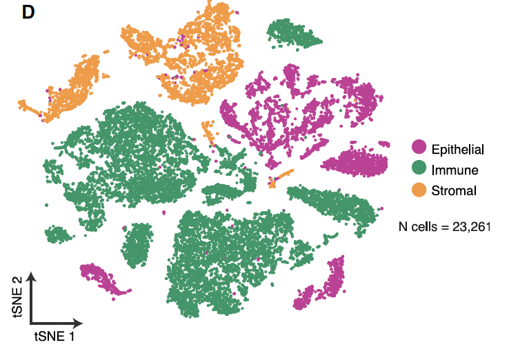
文章提到的各大亚群细胞数量是: (epithelial cells [n = 5,581], immune cells [n = 13,431], stromal cells
[n = 4,249]).
我发现自己怎么都重复不出来,因为唯一的质量控制步骤,细胞数量就开始不吻合了:
 #
 # 这里没有绝对的过滤标准
 # Filter cells so that remaining cells have nGenes >= 500 and nReads >= 50000
 # 26485 features across 27489 samples
 main_tiss_filtered <- subset(x=main_tiss, subset = nCount_RNA > 50000 & nFeature_RNA > 500)
 main_tiss_filtered
 # 26485 features across 21444 samples
也就是说27489个细胞,被过滤成为了 21444细胞,而文章的细胞数量是23261,但是我明明是跟文章作者一模一样的处理过程。
真的是百思不得其解。
后来认真看了看它提供的文件列表:
 1.4G Aug 30 12:04 S01_datafinal.csv
 11M Aug 30 11:34 S01_metacells.csv
 3.5K Aug 30 11:35 by_sample_ratios_driver_muts_3.30.20.csv
 3.3K Aug 30 11:35 neo-osi_metadata.csv
 184M Aug 30 11:35 neo-osi_rawdata.csv
 13K Aug 30 11:34 samples_x_genes_3.30.20.csv
原来是有两个表达矩阵文件,neo-osi_rawdata.csv 和 S01_datafinal.csv 文件,都需要走流程~
需要注意的是这个文章作者并没有上传这些文件到GEO上面,仅仅是上传了原始数据在:https://www.ncbi.nlm.nih.gov/bioproject/?term=PRJNA591860,这个原始数据接近4T的文件。
这些csv文件呢,作者上传到了谷歌云盘,我们人工搬运到了百度云,在交流群可以拿到。如果你也想加入交流群,自己去:你要的rmarkdown文献图表复现全套代码来了(单细胞)找到我们的拉群小助手哈。
我漏掉的这个 neo-osi_rawdata.csv 走流程拿到的是 2070 个单细胞
# 26485 features across 3507 samples within 1 assay
 osi_object_filtered <- subset(x=osi_object, subset = nCount_RNA > 50000 & nFeature_RNA > 500)
 osi_object_filtered
 # 26485 features across 2070 samples within 1 assay
然后把两个单细胞表达矩阵构建好的Seurat 对象合并起来,代码如下:
main_tiss_filtered
osi_object_filtered
main_tiss_filtered1 <- merge(x = main_tiss_filtered, y = osi_object_filtered)
main_tiss_filtered1
得到的就差不多是文章里面的 23514 个单细胞啦,文章的细胞数量是23261。
> main_tiss_filtered1
An object of class Seurat
26485 features across 23514 samples within 1 assay
Active assay: RNA (26485 features, 0 variable features)
全部代码可以复制粘贴的
总共是 270 行,基本上涵盖了我们单细胞天地的方方面面知识点。
rm(list=ls())
options(stringsAsFactors = F)
library(Seurat)
pro='first'

# 单细胞项目:来自于30个病人的49个组织样品,跨越3个治疗阶段

# Single-cell RNA sequencing (scRNA-seq) of
# metastatic lung cancer was performed using 49 clinical biopsies obtained from 30 patients before and during
# targeted therapy.

# before initiating systemic targeted therapy (TKI naive [TN]),
# at the residual disease (RD) state,
# acquired drug resistance (progression [PD]).

# 首先读取第一个单细胞转录组表达矩阵文件:
if(T){

 # Load data
 dir='./'
 Sys.time()
 raw.data <- read.csv(paste(dir,"Data_input/csv_files/S01_datafinal.csv", sep=""), header=T, row.names = 1)
 Sys.time()
 dim(raw.data) #
 raw.data[1:4,1:4]
 head(colnames(raw.data))
 # Load metadata
 metadata <- read.csv(paste(dir,"Data_input/csv_files/S01_metacells.csv", sep=""), row.names=1, header=T)
 head(metadata)

 # Find ERCC's, compute the percent ERCC, and drop them from the raw data.

 erccs <- grep(pattern = "^ERCC-", x = rownames(x = raw.data), value = TRUE)
 percent.ercc <- Matrix::colSums(raw.data[erccs, ])/Matrix::colSums(raw.data)
 fivenum(percent.ercc)
 ercc.index <- grep(pattern = "^ERCC-", x = rownames(x = raw.data), value = FALSE)
 raw.data <- raw.data[-ercc.index,]
 dim(raw.data)
 # Create the Seurat object with all the data (unfiltered)
 main_tiss <- CreateSeuratObject(counts = raw.data)
 # add rownames to metadta
 row.names(metadata) <- metadata$cell_id
 # add metadata to Seurat object
 main_tiss <- AddMetaData(object = main_tiss, metadata = metadata)
 main_tiss <- AddMetaData(object = main_tiss, percent.ercc, col.name = "percent.ercc")
 # Head to check
 head(main_tiss@meta.data)

 # Calculate percent ribosomal genes and add to metadata
 ribo.genes <- grep(pattern = "^RP[SL][[:digit:]]", x = rownames(x = main_tiss@assays$RNA@data), value = TRUE)
 percent.ribo <- Matrix::colSums(main_tiss@assays$RNA@counts[ribo.genes, ])/Matrix::colSums(main_tiss@assays$RNA@data)
 fivenum(percent.ribo)
 main_tiss <- AddMetaData(object = main_tiss, metadata = percent.ribo, col.name = "percent.ribo")
 main_tiss

 # 唯一的质量控制步骤:
 # 这里没有绝对的过滤标准
 # Filter cells so that remaining cells have nGenes >= 500 and nReads >= 50000
 # 26485 features across 27489 samples
 main_tiss_filtered <- subset(x=main_tiss, subset = nCount_RNA > 50000 & nFeature_RNA > 500)
 main_tiss_filtered
 # 26485 features across 21444 samples
}
main_tiss_filtered
# 26485 features across 21444 samples

# 然后读取第二个单细胞转录组表达矩阵文件:
if(T){
 # load and clean rawdata
 # Load data
 dir='./'
 Sys.time()
 osi.raw.data <- read.csv(paste(dir,"Data_input/csv_files/neo-osi_rawdata.csv", sep=""), row.names = 1)

 Sys.time()

 colnames(osi.raw.data) <- gsub("_S.*.homo", "", colnames(osi.raw.data))
 osi.raw.data[1:4,1:4]
 tail( osi.raw.data[ 1:4])
 dim(osi.raw.data)

 # drop sequencing details from gene count table
 # 因为是HTseq这个软件跑出来的表达矩阵
 row.names(osi.raw.data)[grep("__", row.names(osi.raw.data))]
 osi.raw.data <- osi.raw.data[-grep("__", row.names(osi.raw.data)),]

 #Make osi.metadata by cell from osi.metadata by plate

 osi.metadata <- read.csv(paste(dir, "Data_input/csv_files/neo-osi_metadata.csv", sep = ""))
 osi.meta.cell <- as.data.frame(colnames(osi.raw.data))
 osi.meta.cell <- data.frame(do.call('rbind', strsplit(as.character(osi.meta.cell$`colnames(osi.raw.data)`),'_',fixed=TRUE)))
 rownames(osi.meta.cell) <- paste(osi.meta.cell$X1, osi.meta.cell$X2, sep = "_")
 colnames(osi.meta.cell) <- c("well", "plate")
 osi.meta.cell$cell_id <- rownames(osi.meta.cell)
 library(dplyr)
 osi.metadata <- left_join(osi.meta.cell, osi.metadata, by = "plate")
 rownames(osi.metadata) <- osi.metadata$cell_id
 head(osi.metadata)

 unique(osi.metadata$plate)


 # Find ERCC's, compute the percent ERCC, and drop them from the raw data.

 erccs <- grep(pattern = "^ERCC-", x = rownames(x = osi.raw.data), value = TRUE)
 percent.ercc <- Matrix::colSums(osi.raw.data[erccs, ])/Matrix::colSums(osi.raw.data)
 ercc.index <- grep(pattern = "^ERCC-", x = rownames(x = osi.raw.data), value = FALSE)
 osi.raw.data <- osi.raw.data[-ercc.index,]
 dim(osi.raw.data)


 # Create the Seurat object with all the data (unfiltered)

 osi_object <- CreateSeuratObject(counts = osi.raw.data)
 osi_object <- AddMetaData(object = osi_object, metadata = osi.metadata)
 osi_object <- AddMetaData(object = osi_object, percent.ercc, col.name = "percent.ercc")
 # Changing nUMI column name to nReads
 colnames(osi_object@meta.data)[colnames(osi_object@meta.data) == 'nUMI'] <- 'nReads'
 head(osi_object@meta.data)


 # Calculate percent ribosomal genes and add to osi.metadata

 ribo.genes <- grep(pattern = "^RP[SL][[:digit:]]", x = rownames(x = osi_object@assays$RNA@data), value = TRUE)
 percent.ribo <- Matrix::colSums(osi_object@assays$RNA@data[ribo.genes, ])/Matrix::colSums(osi_object@assays$RNA@data)
 osi_object <- AddMetaData(object = osi_object, metadata = percent.ribo, col.name = "percent.ribo")
 osi_object
 # 26485 features across 3507 samples within 1 assay
 osi_object_filtered <- subset(x=osi_object, subset = nCount_RNA > 50000 & nFeature_RNA > 500)
 osi_object_filtered
 # 26485 features across 2070 samples within 1 assay
 VlnPlot(osi_object_filtered, features = "nFeature_RNA")
 VlnPlot(osi_object_filtered, features = "nCount_RNA", log = TRUE)

}
main_tiss_filtered
osi_object_filtered
main_tiss_filtered1 <- merge(x = main_tiss_filtered, y = osi_object_filtered)
main_tiss_filtered1
raw_sce <- main_tiss_filtered1
if(F){
 # Drop any samples with 10 or less cells

 main_tiss_filtered@meta.data$sample_name <- as.character(main_tiss_filtered@meta.data$sample_name)
 sample_name <- as.character(main_tiss_filtered@meta.data$sample_name)
 # Make table
 tab.1 <- table(main_tiss_filtered@meta.data$sample_name)
 # Which samples have less than 10 cells
 samples.keep <- names(which(tab.1 > 10))
 metadata_keep <- filter(main_tiss_filtered@meta.data, sample_name %in% samples.keep)
 # Subset Seurat object
 tiss_subset <- subset(main_tiss_filtered, cells=as.character(metadata_keep$cell_id))
 tiss_subset
 raw_sce <- tiss_subset
}

# Gene-expression profiles of 23,261 cells were retained after quality control filtering.

raw_sce
rownames(raw_sce)[grepl('^mt-',rownames(raw_sce),ignore.case = T)]
rownames(raw_sce)[grepl('^Rp[sl]',rownames(raw_sce),ignore.case = T)]

raw_sce[["percent.mt"]] <- PercentageFeatureSet(raw_sce, pattern = "^MT-")
fivenum(raw_sce[["percent.mt"]][,1])
rb.genes <- rownames(raw_sce)[grep("^RP[SL]",rownames(raw_sce),ignore.case = T)]
C<-GetAssayData(object = raw_sce, slot = "counts")
percent.ribo <- Matrix::colSums(C[rb.genes,])/Matrix::colSums(C)*100
fivenum(percent.ribo)
raw_sce <- AddMetaData(raw_sce, percent.ribo, col.name = "percent.ribo")

plot1 <- FeatureScatter(raw_sce, feature1 = "nCount_RNA", feature2 = "percent.ercc")
plot2 <- FeatureScatter(raw_sce, feature1 = "nCount_RNA", feature2 = "nFeature_RNA")
CombinePlots(plots = list(plot1, plot2))

VlnPlot(raw_sce, features = c("percent.ribo", "percent.ercc"), ncol = 2)
VlnPlot(raw_sce, features = c("nFeature_RNA", "nCount_RNA"), ncol = 2)
VlnPlot(raw_sce, features = c("percent.ribo", "nCount_RNA"), ncol = 2)
raw_sce

sce=raw_sce
sce
#sce <- NormalizeData(sce, normalization.method = "LogNormalize", scale.factor = 1e6)
sce <- NormalizeData(sce, normalization.method = "LogNormalize", scale.factor = 1e5)
GetAssay(sce,assay = "RNA")
sce <- FindVariableFeatures(sce,
 selection.method = "vst", nfeatures = 2000)
# 步骤 ScaleData 的耗时取决于电脑系统配置(保守估计大于一分钟)
sce <- ScaleData(sce)
sce <- RunPCA(object = sce, pc.genes = VariableFeatures(sce))
DimHeatmap(sce, dims = 1:12, cells = 100, balanced = TRUE)
ElbowPlot(sce)
# 跟文章保持一致,第一次分群,resolution 采取 0.5
sce <- FindNeighbors(sce, dims = 1:15)
sce <- FindClusters(sce, resolution = 0.2)
table(sce@meta.data$RNA_snn_res.0.2)
sce <- FindClusters(sce, resolution = 0.8)
table(sce@meta.data$RNA_snn_res.0.8)
sce <- FindClusters(sce, resolution = 0.5)
table(sce@meta.data$RNA_snn_res.0.5)

# 不同的 resolution 分群的结果不一样
library(gplots)
tab.1=table(sce@meta.data$RNA_snn_res.0.2,sce@meta.data$RNA_snn_res.0.8)
balloonplot(tab.1)

# Check clustering stability at given resolution
# Set different resolutions
res.used <- seq(0.1,1,by=0.2)
res.used
# Loop over and perform clustering of different resolutions
for(i in res.used){
 sce <- FindClusters(object = sce, verbose = T, resolution = res.used)
}
# Make plot
library(clustree)
clus.tree.out <- clustree(sce) +
 theme(legend.position = "bottom") +
 scale_color_brewer(palette = "Set1") +
 scale_edge_color_continuous(low = "grey80", high = "red")

clus.tree.out

res.used <- 0.5
sce <- FindClusters(object = sce, verbose = T, resolution = res.used)

set.seed(123)
sce <- RunTSNE(object = sce, dims = 1:15, do.fast = TRUE)
DimPlot(sce,reduction = "tsne",label=T)
phe=data.frame(cell=rownames(sce@meta.data),
 cluster =sce@meta.data$seurat_clusters)
head(phe)
table(phe$cluster)
tsne_pos=Embeddings(sce,'tsne')
head(phe)
table(phe$cluster)
head(tsne_pos)
dat=cbind(tsne_pos,phe)

save(dat,file=paste0(pro,'_for_tSNE.pos.Rdata'))
load(file=paste0(pro,'_for_tSNE.pos.Rdata'))
library(ggplot2)
p=ggplot(dat,aes(x=tSNE_1,y=tSNE_2,color=cluster))+geom_point(size=0.95)
p=p+stat_ellipse(data=dat,aes(x=tSNE_1,y=tSNE_2,fill=cluster,color=cluster),
 geom = "polygon",alpha=0.2,level=0.9,type="t",linetype = 2,show.legend = F)+coord_fixed()
print(p)
theme= theme(panel.grid =element_blank()) + ## 删去网格
 theme(panel.border = element_blank(),panel.background = element_blank()) + ## 删去外层边框
 theme(axis.line = element_line(size=1, colour = "black"))
p=p+theme+guides(colour = guide_legend(override.aes = list(size=5)))
print(p)
ggplot2::ggsave(filename = paste0(pro,'_tsne.pdf'))

sce <- RunUMAP(object = sce, dims = 1:15, do.fast = TRUE)
DimPlot(sce,reduction = "umap",label=T)
ggplot2::ggsave(filename = paste0(pro,'_umap.pdf'))

sce.markers <- FindAllMarkers(object = sce, only.pos = TRUE, min.pct = 0.25,
 thresh.use = 0.25)

DT::datatable(sce.markers)
write.csv(sce.markers,file=paste0(pro,'_sce.markers.csv'))
library(dplyr)
top10 <- sce.markers %>% group_by(cluster) %>% top_n(10, avg_logFC)
DoHeatmap(sce,top10$gene,size=3)
ggsave(filename=paste0(pro,'_sce.markers_heatmap.pdf'))
sce.first=sce
save(sce.first,sce.markers,file = 'first_sce.Rdata')
如果你看不懂代码,请自行回顾:单细胞基础10讲
- 01. 上游分析流程
- 02.课题多少个样品,测序数据量如何
- 03. 过滤不合格细胞和基因(数据质控很重要)
- 04. 过滤线粒体核糖体基因
- 05. 去除细胞效应和基因效应
- 06.单细胞转录组数据的降维聚类分群
- 07.单细胞转录组数据处理之细胞亚群注释
- 08.把拿到的亚群进行更细致的分群
- 09.单细胞转录组数据处理之细胞亚群比例比较
更多个性化汇总代码见:单细胞初级8讲和高级分析8讲
初级分析
- 单细胞转录组基础分析一:分析环境搭建
- 单细胞转录组基础分析二:数据质控与标准化
- 单细胞转录组基础分析三:降维与聚类
- 单细胞转录组基础分析四:细胞类型鉴定
- 单细胞转录组基础分析五:细胞再聚类
- 单细胞转录组基础分析六:伪时间分析
- 单细胞转录组基础分析七:差异基因富集分析
- 单细胞转录组基础分析八:可视化工具总结