单细胞转录组虽然说不太可能跟传统的bulk转录组那样对每个样本都测定到好几万基因的表达量,如果是10x这样的技术,每个细胞也就几百个基因是有表达量的,但是架不住细胞数量多,对大量细胞来说,这个表达矩阵的基因数量就很可观了。一般来说,gencode数据库的gtf文件注释到的五万多个基因里面,包括蛋白编码基因和非编码的,可以在单细胞表达矩阵里面过滤低表达量后,还剩下2万多个左右。
2万个基因,近万个细胞的表达矩阵,降维起来是一个浩大的计算量,所以有一个步骤,就是从2万个基因里面挑选一下 highly variable genes (HVG) 进行下游分析,从此就假装自己的单细胞转录组就仅仅是测到了HVGs,数量嘛,两千多吧!
那么,问题就来了, 什么样的标准算法来挑选 highly variable genes (HVG) 进行下游分析呢?
搜索最新文献
简单谷歌搜索highly variable genes (HVG) 加上单细胞,这样的关键词就可以看到很多手把手教程:
- 2019六月的:Current best practices in single‐cell RNA‐seq analysis: a tutorial 地址:https://www.embopress.org/doi/10.15252/msb.20188746
- bioconductor教程:Using scran to analyze single-cell RNA-seq data https://bioconductor.org/packages/devel/bioc/vignettes/scran/inst/doc/scran.html
- 一步步手把手流程:https://dockflow.org/workflow/simple-single-cell/
基本上经过四五个小时的模式,你就会总结到一些常见的挑选 highly variable genes (HVG) 的算法和R包,我简单罗列5个,会对比一下:
- seurat包的FindVariableFeatures函数,默认挑选2000个
- monocle包的monocle_hvg函数
- scran包的decomposeVar函数
- M3Drop的BrenneckeGetVariableGenes
- 以及文献参考::(Brennecke et al 2013 method) Extract genes with a squared coefficient of variation >2 times the fit regression
在scRNAseq数据集比较这5个方法
接下来我就没有空继续做这些琐碎的比较啦,老规矩,跟我们的单细胞一期和二期视频学习一下,学习笔记我们有专员操刀,下面看公司学习者的表演:
目的:利用scRNA-seq包的表达矩阵测试几个R包寻找HVGs,然后画upsetR图看看不同方法的HVG的重合情况。
rm(list = ls())
options(stringsAsFactors = F)
关于测试数据scRNAseq
包中内置了Pollen et al. 2014 的数据集(https://www.nature.com/articles/nbt.2967),到19年8月为止,已经有446引用量了。只不过原文完整的数据是 23730 features, 301 samples,这个包中只选取了4种细胞类型:pluripotent stem cells 分化而成的 neural progenitor cells (NPC,神经前体细胞) ,还有 GW16(radial glia,放射状胶质细胞) 、GW21(newborn neuron,新生儿神经元) 、GW21+3(maturing neuron,成熟神经元)
library(scRNAseq)
## ----- Load Example Data -----
data(fluidigm)

# 得到RSEM矩阵
assay(fluidigm) <- assays(fluidigm)$rsem_counts
ct <- floor(assays(fluidigm)$rsem_counts)
ct[1:4,1:4]
## SRR1275356 SRR1274090 SRR1275251 SRR1275287
## A1BG 0 0 0 0
## A1BG-AS1 0 0 0 0
## A1CF 0 0 0 0
## A2M 0 0 0 33
# 样本注释信息
pheno_data <- as.data.frame(colData(fluidigm))
table(pheno_data$Coverage_Type)
##
## High Low
## 65 65
table(pheno_data$Biological_Condition)
##
## GW16 GW21 GW21+3 NPC
## 52 16 32 30
利用Seurat V3
suppressMessages(library(Seurat))
packageVersion("Seurat") # 检查版本信息
## [1] '3.0.2'
seurat_sce <- CreateSeuratObject(counts = ct,
 meta.data = pheno_data,
 min.cells = 5,
 min.features = 2000,
 project = "seurat_sce")
seurat_sce <- NormalizeData(seurat_sce)
# 默认取前2000个
seurat_sce <- FindVariableFeatures(seurat_sce, selection.method = "vst", nfeatures=2000)
VariableFeaturePlot(seurat_sce)
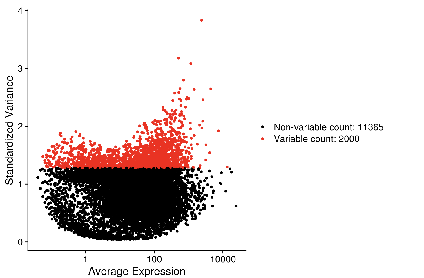
seurat_hvg <- VariableFeatures(seurat_sce)
length(seurat_hvg)
## [1] 2000
head(seurat_hvg)
## [1] "FOS" "ERBB4" "SCD" "SGPL1" "ARID5B" "IGFBPL1"
利用Monocle
library(monocle)
gene_ann <- data.frame(
 gene_short_name = row.names(ct),
 row.names = row.names(ct)
)
sample_ann <- pheno_data
# 然后转换为AnnotatedDataFrame对象
pd <- new("AnnotatedDataFrame",
 data=sample_ann)
fd <- new("AnnotatedDataFrame",
 data=gene_ann)
monocle_cds <- newCellDataSet(
 ct,
 phenoData = pd,
 featureData =fd,
 expressionFamily = negbinomial.size(),
 lowerDetectionLimit=1)
monocle_cds
## CellDataSet (storageMode: environment)
## assayData: 26255 features, 130 samples
## element names: exprs
## protocolData: none
## phenoData
## sampleNames: SRR1275356 SRR1274090 ... SRR1275261 (130 total)
## varLabels: NREADS NALIGNED ... Size_Factor (29 total)
## varMetadata: labelDescription
## featureData
## featureNames: A1BG A1BG-AS1 ... ZZZ3 (26255 total)
## fvarLabels: gene_short_name
## fvarMetadata: labelDescription
## experimentData: use 'experimentData(object)'
## Annotation:
monocle_cds <- estimateSizeFactors(monocle_cds)
monocle_cds <- estimateDispersions(monocle_cds)
disp_table <- dispersionTable(monocle_cds)
unsup_clustering_genes <- subset(disp_table, mean_expression >= 0.1)
monocle_cds <- setOrderingFilter(monocle_cds, unsup_clustering_genes$gene_id)
plot_ordering_genes(monocle_cds)
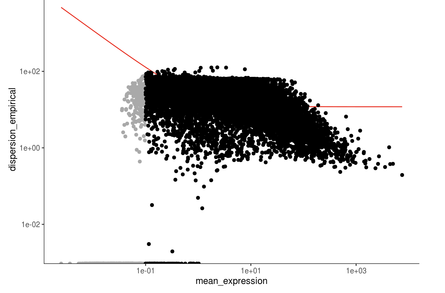
monocle_hvg <- unsup_clustering_genes[order(unsup_clustering_genes$mean_expression, decreasing=TRUE),][,1]
length(monocle_hvg)
## [1] 13986
# 也取前2000个
monocle_hvg <- monocle_hvg[1:2000]
head(monocle_hvg)
## [1] "MALAT1" "TUBA1A" "MAP1B" "SOX4" "EEF1A1" "SOX11"
利用scran
library(SingleCellExperiment)
library(scran)
scran_sce <- SingleCellExperiment(list(counts=ct))
scran_sce <- computeSumFactors(scran_sce)
scran_sce <- normalize(scran_sce)
fit <- trendVar(scran_sce, parametric=TRUE,use.spikes=FALSE)
dec <- decomposeVar(scran_sce, fit)

plot(dec$mean, dec$total, xlab="Mean log-expression",
 ylab="Variance of log-expression", pch=16)
curve(fit$trend(x), col="dodgerblue", add=TRUE)
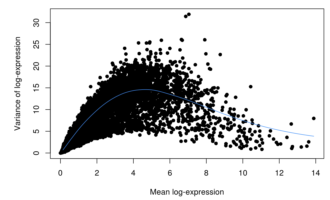
scran_df <- dec
scran_df <- scran_df[order(scran_df$bio, decreasing=TRUE),]
scran_hvg <- rownames(scran_df)[scran_df$FDR<0.1]
length(scran_hvg)
## [1] 875
head(scran_hvg)
## [1] "IGFBPL1" "STMN2" "ANP32E" "EGR1" "DCX" "XIST"
利用M3Drop
library(M3DExampleData)
# 需要提供表达矩阵(expr_mat)=》normalized or raw (not log-transformed)
HVG <-M3Drop::BrenneckeGetVariableGenes(expr_mat=ct, spikes=NA, suppress.plot=FALSE, fdr=0.1, minBiolDisp=0.5, fitMeanQuantile=0.8)
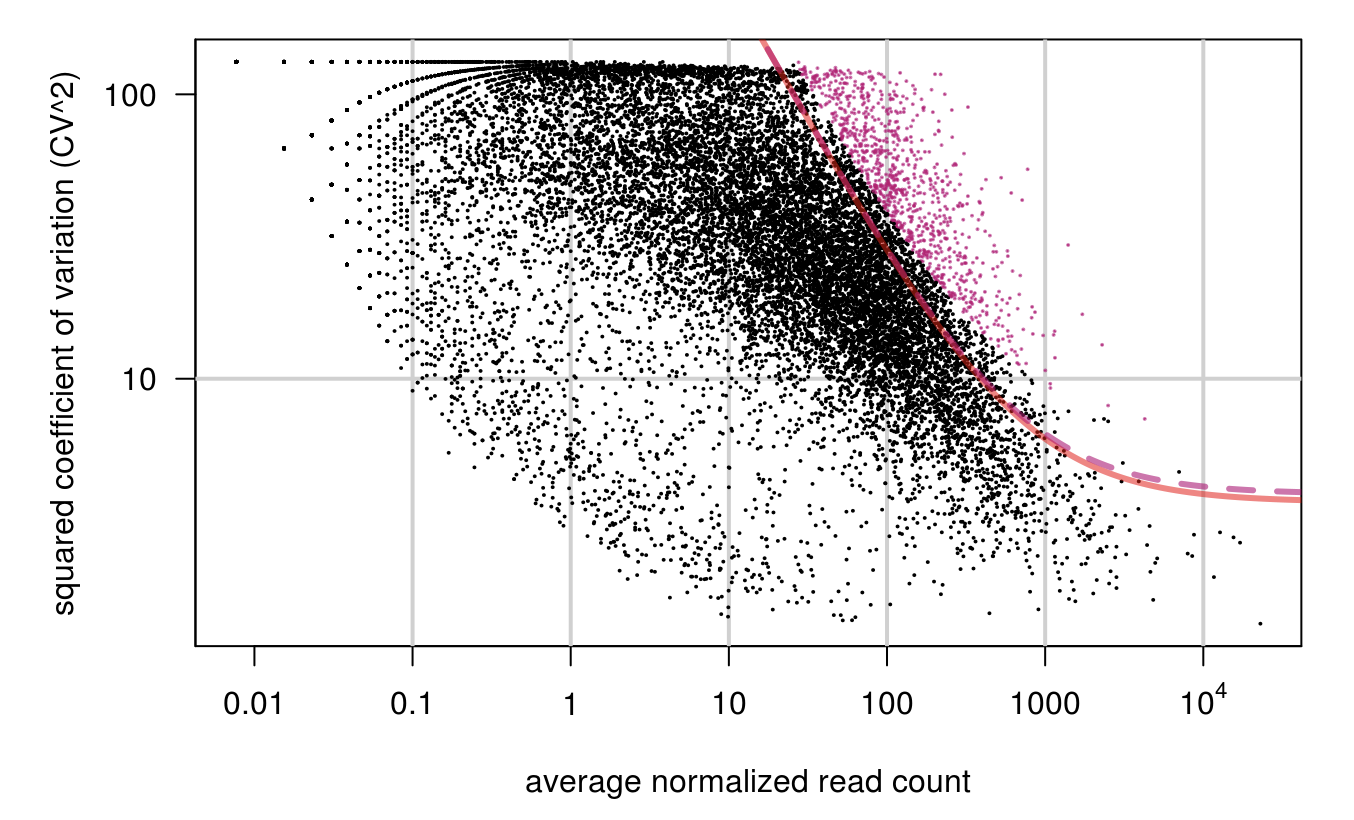
M3Drop_hvg <- rownames(HVG)
length(M3Drop_hvg)
## [1] 917
head(M3Drop_hvg)
## [1] "CCL2" "EMP1" "ZNF630" "NRDE2" "PLCL1" "KCTD21"
自定义函数
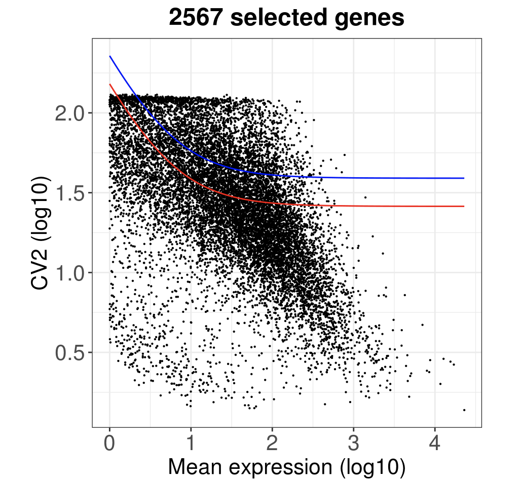
来自:(Brennecke et al 2013 method) Extract genes with a squared coefficient of variation >2 times the fit regression
实现了:Select the highly variable genes based on the squared coefficient of variation and the mean gene expression and return the RPKM matrix the the HVG
if(T){
 getMostVarGenes <- function(
 data=data, # RPKM matrix
 fitThr=1.5, # Threshold above the fit to select the HGV
 minMeanForFit=1 # Minimum mean gene expression level
 ){
 # data=females;fitThr=2;minMeanForFit=1
 # Remove genes expressed in no cells
 data_no0 <- as.matrix(
 data[rowSums(data)>0,]
 )
 # Compute the mean expression of each genes
 meanGeneExp <- rowMeans(data_no0)
 names(meanGeneExp)<- rownames(data_no0)

# Compute the squared coefficient of variation
 varGenes <- rowVars(data_no0)
 cv2 <- varGenes / meanGeneExp^2

# Select the genes which the mean expression is above the expression threshold minMeanForFit
 useForFit <- meanGeneExp >= minMeanForFit

# Compute the model of the CV2 as a function of the mean expression using GLMGAM
 fit <- glmgam.fit( cbind( a0 = 1,
 a1tilde = 1/meanGeneExp[useForFit] ),
 cv2[useForFit] )
 a0 <- unname( fit$coefficients["a0"] )
 a1 <- unname( fit$coefficients["a1tilde"])

# Get the highly variable gene counts and names
 fit_genes <- names(meanGeneExp[useForFit])
 cv2_fit_genes <- cv2[useForFit]
 fitModel <- fit$fitted.values
 names(fitModel) <- fit_genes
 HVGenes <- fitModel[cv2_fit_genes>fitModel*fitThr]
 print(length(HVGenes))

# Plot the result
 plot_meanGeneExp <- log10(meanGeneExp)
 plot_cv2 <- log10(cv2)
 plotData <- data.frame(
 x=plot_meanGeneExp[useForFit],
 y=plot_cv2[useForFit],
 fit=log10(fit$fitted.values),
 HVGenes=log10((fit$fitted.values*fitThr))
 )
 p <- ggplot(plotData, aes(x,y)) +
 geom_point(size=0.1) +
 geom_line(aes(y=fit), color="red") +
 geom_line(aes(y=HVGenes), color="blue") +
 theme_bw() +
 labs(x = "Mean expression (log10)", y="CV2 (log10)")+
 ggtitle(paste(length(HVGenes), " selected genes", sep="")) +
 theme(
 axis.text=element_text(size=16),
 axis.title=element_text(size=16),
 legend.text = element_text(size =16),
 legend.title = element_text(size =16 ,face="bold"),
 legend.position= "none",
 plot.title = element_text(size=18, face="bold", hjust = 0.5),
 aspect.ratio=1
 )+
 scale_color_manual(
 values=c("#595959","#5a9ca9")
 )
 print(p)

# Return the RPKM matrix containing only the HVG
 HVG <- data_no0[rownames(data_no0) %in% names(HVGenes),]
 return(HVG)
 }
}
library(statmod)
diy_hvg <- rownames(getMostVarGenes(ct))
## [1] 2567
看起来代码比较长,主要是绘图的时候拖拉了。
length(diy_hvg)
## [1] 2567
head(diy_hvg)
## [1] "A2M" "A2MP1" "AAMP" "ABCA11P" "ABCA3" "ABCB10"
upsetR作图
require(UpSetR)
input <- fromList(list(seurat=seurat_hvg, monocle=monocle_hvg,
 scran=scran_hvg, M3Drop=M3Drop_hvg, diy=diy_hvg))
upset(input)
很多图都是可以美化的,不过并不是我们的重点
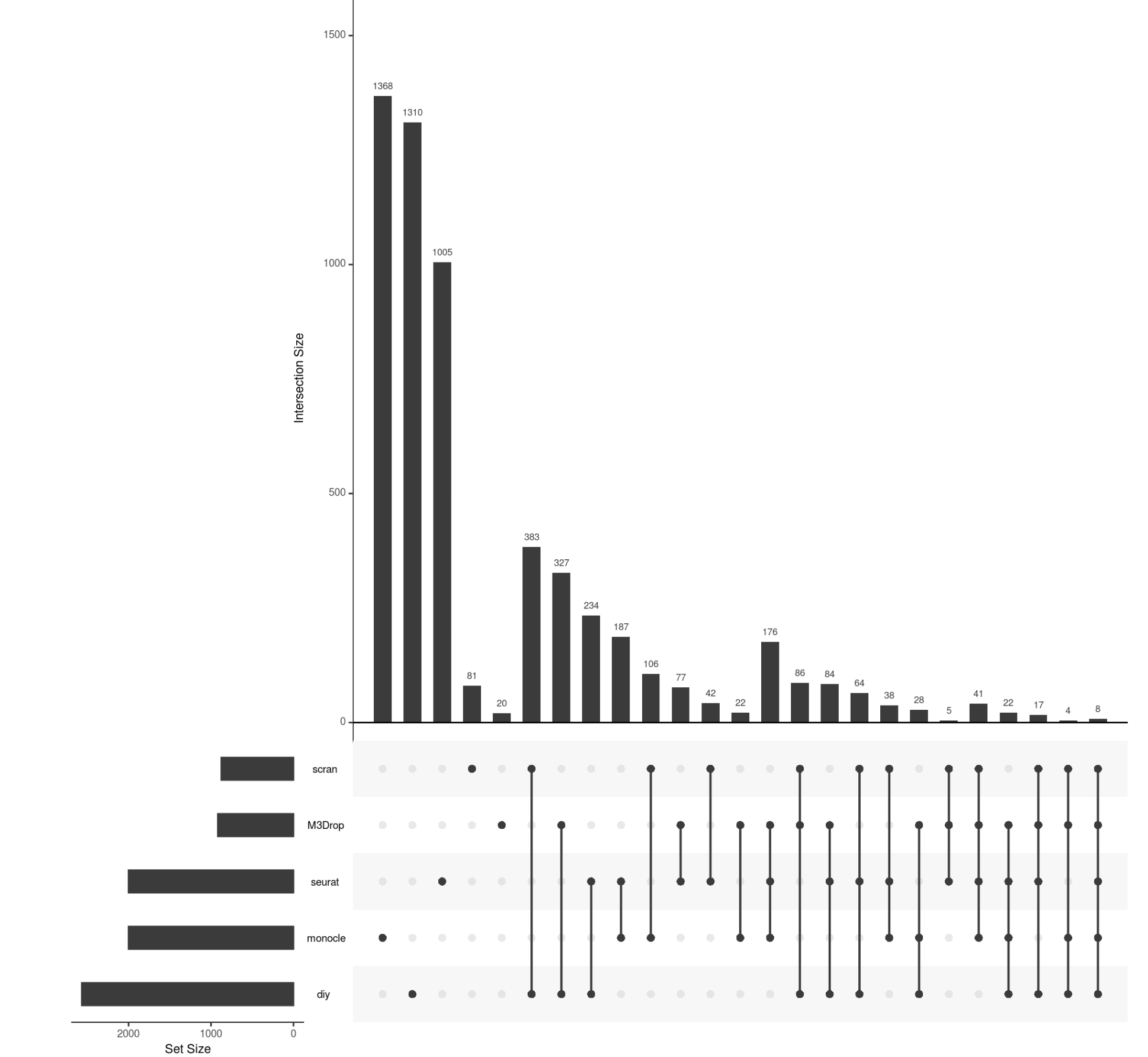
可以看到,不同的R包和方法,差异不是一般的大啊!!!
更多方法
比如基尼系数:findHVG: Finding highly variable genes (HVG) based on Gini 见:https://rdrr.io/github/jingshuw/descend/man/findHVG.html
赶快试一下吧,探索的过程中,你就会对单细胞数据处理的认知加强了。