昨天我在生信菜鸟团分享的学徒数据挖掘任务: 不一定正确的多分组差异分析结果热图展现 提到了可以使用单细胞转录组数据分析流程来处理文献的数据集。
还给出了一些简单代码,就是看看样本聚类情况,然后留下作业给另外一个学徒,看单细胞R包Seurat的FindAllMarkers函数对7个亚型找到的marker基因,根据传统的bulk转录组差异分析策略的差异。
先看看单细胞转录组代码
这里我们的单细胞转录组数据分析方法,基本上遵循我的全网第一个单细胞课程(基础)满一千份销量就停止发售 内容,就是一些R包的认知,包括 scater,monocle,Seurat,scran,M3Drop 需要熟练掌握它们的对象,:一些单细胞转录组R包的对象 ,分析流程也大同小异:
- step1: 创建对象
- step2: 质量控制
- step3: 表达量的标准化和归一化
- step4: 去除干扰因素(多个样本整合)
- step5: 判断重要的基因
- step6: 多种降维算法
- step7: 可视化降维结果
- step8: 多种聚类算法
- step9: 聚类后找每个细胞亚群的标志基因
- step10: 继续分类
代码如下:
library(Seurat)
# https://satijalab.org/seurat/mca.html
sce <- CreateSeuratObject(counts = sarc_choose,
meta.data =clinic,
min.cells = 5, min.features = 1000,
project = "sce")
head(sce@meta.data)
# 步骤 ScaleData 的耗时取决于电脑系统配置(保守估计大于一分钟)
sce <- ScaleData(object = sce,
vars.to.regress = c('nCount_RNA'),
model.use = 'linear',
use.umi = FALSE)
sce <- FindVariableFeatures(object = sce,
mean.function = ExpMean,
dispersion.function = LogVMR,
x.low.cutoff = 0.0125,
x.high.cutoff = 4,
y.cutoff = 0.5)
length(VariableFeatures(sce))
sce <- RunPCA(object = sce, pc.genes = VariableFeatures(sce))
# 下面只是展现不同降维算法而已,并不要求都使用一次。
sce <- RunICA(sce )
sce <- RunTSNE(sce )
#sce <- RunUMAP(sce,dims = 1:10)
#VizPCA( sce, pcs.use = 1:2)
DimPlot(object = sce, reduction = "pca")
DimPlot(object = sce, reduction = "ica")
DimPlot(object = sce, reduction = "tsne",group.by = 'short.histo')
# 针对PCA降维后的表达矩阵进行聚类 FindNeighbors+FindClusters 两个步骤。
sce <- FindNeighbors(object = sce, dims = 1:20, verbose = FALSE)
sce <- FindClusters(object = sce, resolution = 0.8,verbose = FALSE)
# 继续tSNE可视化
DimPlot(object = sce, reduction = "tsne",
group.by = 'RNA_snn_res.0.8',label = T)
table(sce@meta.data$short.histo,sce@meta.data$RNA_snn_res.0.8)
Idents(sce)=sce@meta.data$short.histo
sce.markers <- FindAllMarkers(object = sce, only.pos = TRUE, min.pct = 0.25,
thresh.use = 0.25)
DT::datatable(sce.markers)
library(dplyr)
sce.markers=sce.markers[!is.infinite(sce.markers$avg_logFC),]
sce.markers %>% group_by(cluster) %>% top_n(2, avg_logFC)
topN <- sce.markers %>% group_by(cluster) %>% top_n(50, avg_logFC)
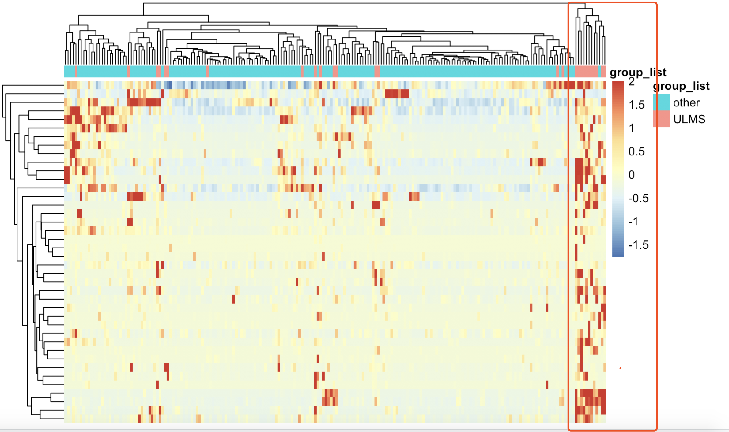
DoHeatmap(sce,topN$gene)
热图如下:

可以看到R包Seurat的FindAllMarkers函数对7个亚型找到的marker基因基本上都是上调基因。
检查单细胞转录组和bulk差异分析结果重合情况
首先bulk差异分析策略见: 不一定正确的多分组差异分析结果热图展现 ,其实就是我们以前在生信技能树分享的一个策略:如果你的分组比较多,差异分析策略有哪些? 把其中一个亚型跟所有的其它样本进行常规转录组差异分析而已。差异分析结果如下:
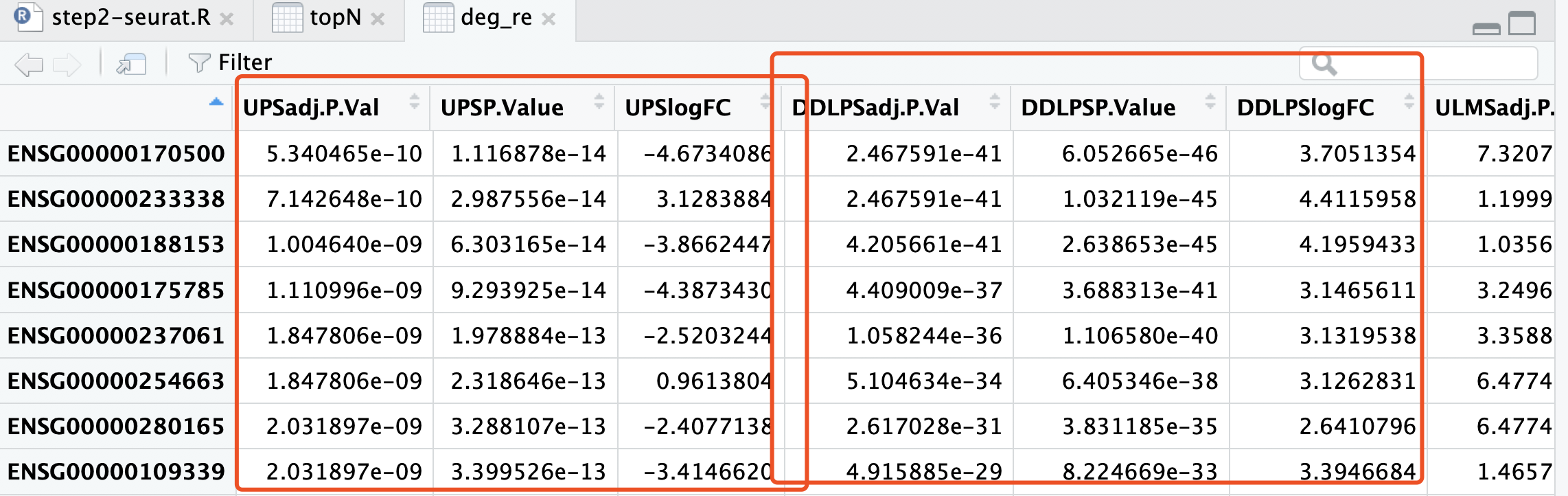
我们的单细胞转录组分析结果的,topN 这个变量,就存储着其差异分析结果:
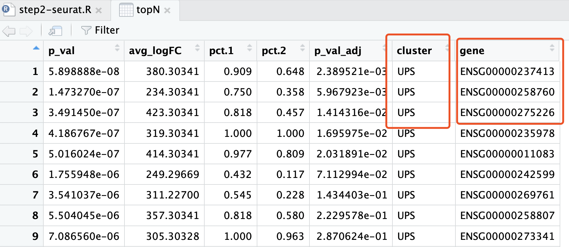
现在要比较这两个表格!
单细胞FindAllMarkers并不是简单取差异最大的基因
通常,我们对传统bulk转录组差异分析结果,可以选取top的上下调基因进行热图可视化,如下:

但是,我们上面单细胞流程的R包Seurat的FindAllMarkers函数对ULMS亚型找到的marker基因,却并不满足这个传统bulk转录组差异分析统计学显著指标,比如logFC大于2,并且校正后的P值小于0.05
不过,也是可以看到这样的规律,就是挑选的基因可以显著的把绝大部分ULMS 亚型病人跟其他病人区分开来。
但是,这些基因,在limma的voom算法的差异分析结果里面,只有非常少的几个基因的阈值是达标的:
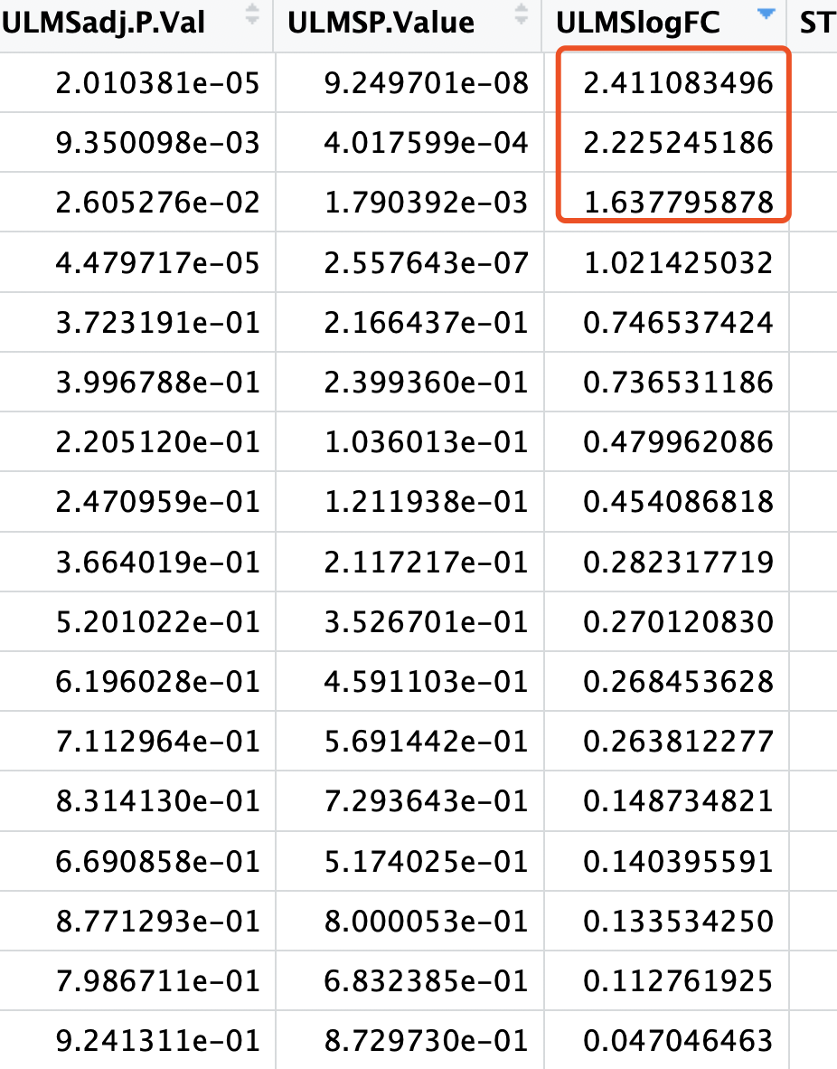
绝大部分基因的logFC机会没有啥意义。
其实FindAllMarkers找基因还有很多参数可以选择
有趣的是,就是没有limma的voom算法!
"wilcox" : Identifies differentially expressed genes between two groups of cells using a Wilcoxon Rank Sum test (default)
"bimod" : Likelihood-ratio test for single cell gene expression, (McDavid et al., Bioinformatics, 2013)
"roc" : Identifies 'markers' of gene expression using ROC analysis. For each gene, evaluates (using AUC) a classifier built on that gene alone, to classify between two groups of cells. An AUC value of 1 means that expression values for this gene alone can perfectly classify the two groupings (i.e. Each of the cells in cells.1 exhibit a higher level than each of the cells in cells.2). An AUC value of 0 also means there is perfect classification, but in the other direction. A value of 0.5 implies that the gene has no predictive power to classify the two groups. Returns a 'predictive power' (abs(AUC-0.5) * 2) ranked matrix of putative differentially expressed genes.
"t" : Identify differentially expressed genes between two groups of cells using the Student's t-test.
"negbinom" : Identifies differentially expressed genes between two groups of cells using a negative binomial generalized linear model. Use only for UMI-based datasets
"poisson" : Identifies differentially expressed genes between two groups of cells using a poisson generalized linear model. Use only for UMI-based datasets
"LR" : Uses a logistic regression framework to determine differentially expressed genes. Constructs a logistic regression model predicting group membership based on each feature individually and compares this to a null model with a likelihood ratio test.
"MAST" : Identifies differentially expressed genes between two groups of cells using a hurdle model tailored to scRNA-seq data. Utilizes the MAST package to run the DE testing.
"DESeq2" : Identifies differentially expressed genes between two groups of cells based on a model using DESeq2 which uses a negative binomial distribution (Love et al, Genome Biology, 2014).This test does not support pre-filtering of genes based on average difference (or percent detection rate) between cell groups. However, genes may be pre-filtered based on their minimum detection rate (min.pct) across both cell groups. To use this method, please install DESeq2, using the instructions at https://bioconductor.org/packages/release/bioc/html/DESeq2.html
感兴趣的朋友,可以一一尝试,当然了,还不如系统性学习下统计学知识哦
可是,统计学不比尝试这些参数要简单其实。