首先要明白这个ES score图片里面的数据是什么,这样才能修改它,因为java是一个封闭打包好的软件,所以我们没办法在里面修改它没有提供的参数,运行完GSEA,默认输出的图就是下面这样:
ES score
这个图片在发表的时候,就会发现其实蛮模糊的, 所以有可能需要自己重新制作这个图,那么就需要明白这个图后面的数据。
其中最下面的数据是量方法测到了2万个基因,那么这两万个基因在case和control组的差异度量(六种差异度量,默认是signal 2 noise,GSEA官网有提供公式,也可以选择大家熟悉的foldchange)肯定不一样,那么根据它们的差异度量,就可以对它们进行排序,并且Z-score标准化的结果。
而中间的就是该gene set在测到了的已经根据signal2noise排好序的2万个基因的位置。
最上面的图,就是所有的基因的ES score都要一个个加起来,叫做running ES score,在加的过程中,什么时候ES score达到了最大值,就是这个gene set最终的ES score!
我这里全面解析了GSEA官网提供的R代码的绘图函数,如下:
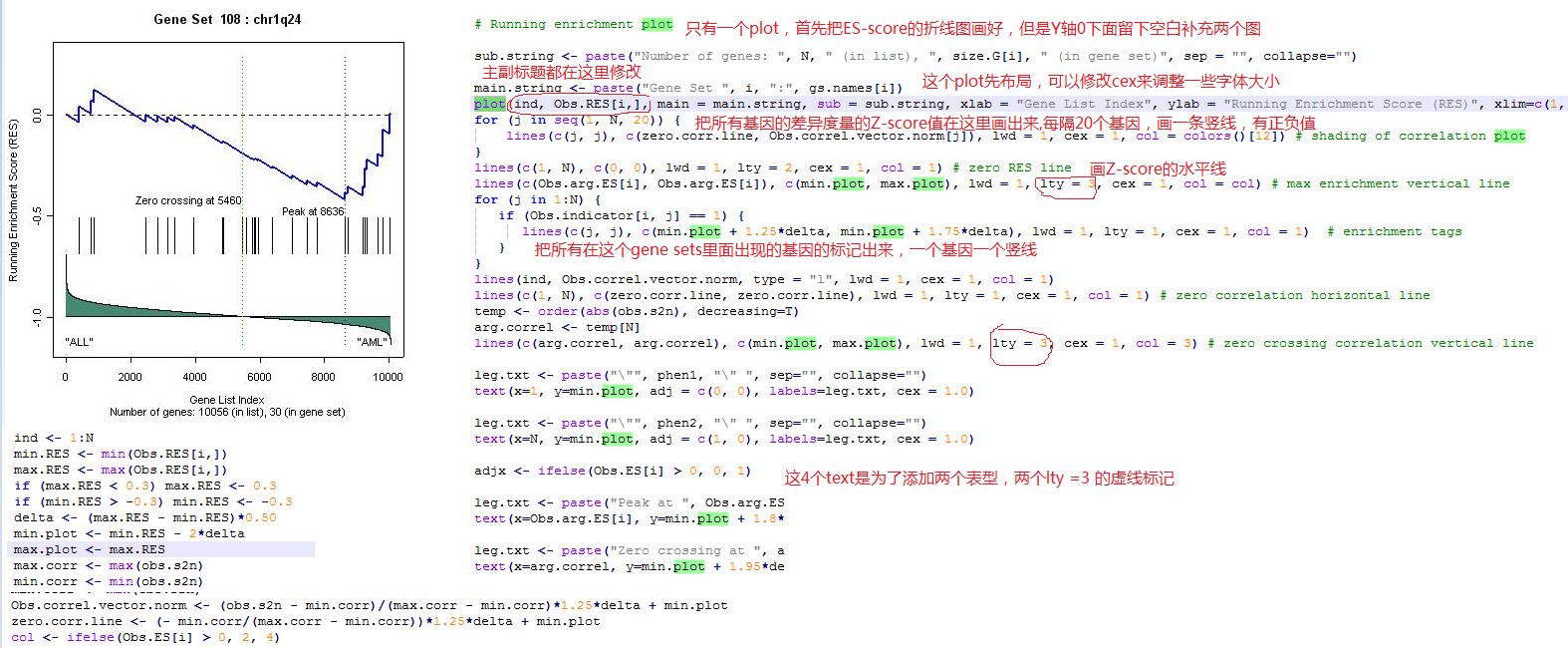
这个函数本身也被我抽离出来了:
这个知识点有点复杂,我解释的很清楚数据是什么,但是数据如何来的(就是下面代码读取的txt文件),我没办法用博客写清楚,需要修改一个2500行的源代码才能获取数据!
setwd('data')
Obs.RES=read.table('Obs.RES.txt')
Obs.RES=t(Obs.RES) ## 每个基因在每个gene set里面的running ES score,一个矩阵
Obs.indicator=read.table('Obs.indicator.txt')
Obs.indicator=t(Obs.indicator) ## 每个基因是否属于每个gene set,一个0/1矩阵
obs.s2n=read.table('obs.s2n.txt')[,1] ## 每个基因的signal 2 noise值,已经Z-score化,而且排好序了。
size.G=read.table('size.G.txt')[,1] ## 每个gene set的基因数量,在图中需要显示
gs.names=read.table('gs.names.txt')[,1] ## 每个gene set的名字,在图中需要显示
Obs.arg.ES=read.table('Obs.arg.ES.txt')[,1]## 每个gene set的最大ES score出现在排序基因的位置
Obs.ES.index=read.table('Obs.ES.index.txt')[,1]## 这个用不着的,我也忘记是什么了
Obs.ES=read.table('Obs.ES.txt')[,1] ##每个gene set的最大ES score是多少,如果是正值,用红色表示富集在case组,如果是负值,用蓝色,表示富集在control组。plot_ES_score <- function(Ng=12,N=34688,phen1='control',phen2='case',Obs.RES,Obs.indicator,obs.s2n,size.G,gs.names,Obs.arg.ES,Obs.ES.index){
for (i in 1:Ng) {
png(paste0('number_',gs.names[i],'.png'))
ind <- 1:N
min.RES <- min(Obs.RES[i,])
max.RES <- max(Obs.RES[i,])
if (max.RES < 0.3) max.RES <- 0.3
if (min.RES > -0.3) min.RES <- -0.3
delta <- (max.RES - min.RES)*0.50
min.plot <- min.RES - 2*delta
max.plot <- max.RES
max.corr <- max(obs.s2n)
min.corr <- min(obs.s2n)
Obs.correl.vector.norm <- (obs.s2n - min.corr)/(max.corr - min.corr)*1.25*delta + min.plot
zero.corr.line <- (- min.corr/(max.corr - min.corr))*1.25*delta + min.plot
col <- ifelse(Obs.ES[i] > 0, 2, 4)# Running enrichment plot
sub.string <- paste("Number of genes: ", N, " (in list), ", size.G[i], " (in gene set)", sep = "", collapse="")
main.string <- paste("Gene Set ", i, ":", gs.names[i])
plot(ind, Obs.RES[i,], main = main.string, sub = sub.string, xlab = "Gene List Index", ylab = "Running Enrichment Score (RES)", xlim=c(1, N), ylim=c(min.plot, max.plot), type = "l", lwd = 2, cex = 1, col = col)
for (j in seq(1, N, 20)) {
lines(c(j, j), c(zero.corr.line, Obs.correl.vector.norm[j]), lwd = 1, cex = 1, col = colors()[12]) # shading of correlation plot
}
lines(c(1, N), c(0, 0), lwd = 1, lty = 2, cex = 1, col = 1) # zero RES line
lines(c(Obs.arg.ES[i], Obs.arg.ES[i]), c(min.plot, max.plot), lwd = 1, lty = 3, cex = 1, col = col) # max enrichment vertical line
for (j in 1:N) {
if (Obs.indicator[i, j] == 1) {
lines(c(j, j), c(min.plot + 1.25*delta, min.plot + 1.75*delta), lwd = 1, lty = 1, cex = 1, col = 1) # enrichment tags
}
}
lines(ind, Obs.correl.vector.norm, type = "l", lwd = 1, cex = 1, col = 1)
lines(c(1, N), c(zero.corr.line, zero.corr.line), lwd = 1, lty = 1, cex = 1, col = 1) # zero correlation horizontal line
temp <- order(abs(obs.s2n), decreasing=T)
arg.correl <- temp[N]
lines(c(arg.correl, arg.correl), c(min.plot, max.plot), lwd = 1, lty = 3, cex = 1, col = 3) # zero crossing correlation vertical lineleg.txt <- paste("\"", phen1, "\" ", sep="", collapse="")
text(x=1, y=min.plot, adj = c(0, 0), labels=leg.txt, cex = 1.0)leg.txt <- paste("\"", phen2, "\" ", sep="", collapse="")
text(x=N, y=min.plot, adj = c(1, 0), labels=leg.txt, cex = 1.0)adjx <- ifelse(Obs.ES[i] > 0, 0, 1)
leg.txt <- paste("Peak at ", Obs.arg.ES[i], sep="", collapse="")
text(x=Obs.arg.ES[i], y=min.plot + 1.8*delta, adj = c(adjx, 0), labels=leg.txt, cex = 1.0)leg.txt <- paste("Zero crossing at ", arg.correl, sep="", collapse="")
text(x=arg.correl, y=min.plot + 1.95*delta, adj = c(adjx, 0), labels=leg.txt, cex = 1.0)
dev.off()
}}
通过这个代码,就可以把当前所有gese set的 ES score图给重新画一下,如果需要调整字体大小,就去代码里面慢慢调整。