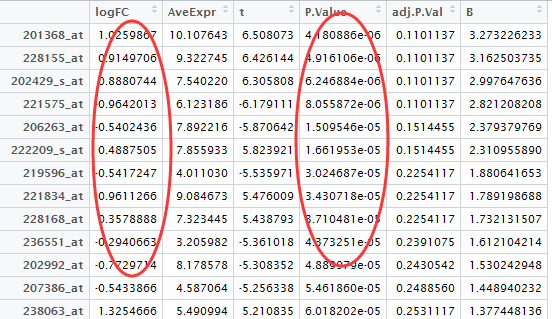
十二 30

用GSEA来做基因集富集分析

how to use GSEA?
这个有点类似于pathway(GO,KEGG等)的富集分析,区别在于gene set(矫正好的基于文献的数据库)的概念更广泛一点,包括了

how to download GSEA ?

what's the input for the GSEA?

说明书上写的输入数据是:GSEA supported data files are simply tab delimited ASCII text files, which have special file extensions that identify them. For example, expression data usually has the extension *.gct, phenotypes *.cls, gene sets *.gmt, and chip annotations *.chip. Click the More on file formats help button to view detailed descriptions of all the data file formats.
实际上没那么复杂,一个表达矩阵即可!然后做一个分组说明的cls文件即可。
主要是自己看说明书,做出要求的数据格式:http://www.broadinstitute.org/cancer/software/gsea/wiki/index.php/Data_formats
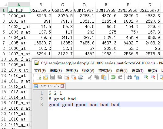
表达矩阵我这里下载GSE1009数据集做测试吧!
cls的样本说明文件,就随便搞一搞吧,下面这个是例子:
6 2 1
# good bad
good good good bad bad bad
文件如下,六个样本,根据探针来的表达数据,分组前后各三个一组。
clipboard
现在开始运行GSEA!

start to run the GSEA !

首先载入数据
clipboard
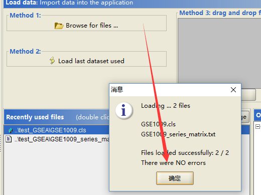
确定无误,就开始运行,运行需要设置一定的参数!
clipboard

what's the output ?

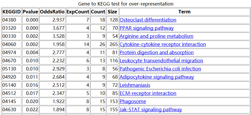
输出的数据非常多,对你选择的gene set数据集里面的每个set都会分析看看是否符合富集的标准,富集就出来一个报告。
点击success就能进入报告主页,里面的链接可以进入任意一个分报告。
最大的特色是提供了大量的数据集:You can browse the MSigDB from the Molecular Signatures Database page of the GSEA web site or the Browse MSigDB page of the GSEA application. To browse the MSigDB from the GSEA application:
 
有些文献是基于GSEA的:


十二 15

用超几何分布检验做富集分析

我们可以直接使用R的bioconductor里面的一个包,GOstats里面的函数来做超几何分布检验,看看每条pathway是否会富集

我们直接读取用limma包做好的差异分析结果

setwd("D:\\my_tutorial\\补\\用limma包对芯片数据做差异分析")

DEG=read.table("GSE63067.diffexp.NASH-normal.txt",stringsAsFactors = F)

View(DEG)

image001

我们挑选logFC的绝对值大于0.5,并且P-value小雨0.05的基因作为差异基因,并且转换成entrezID

probeset=rownames(DEG[abs(DEG[,1])>0.5 & DEG[,4]<0.05,])

library(hgu133plus2.db)

library(annotate)

platformDB="hgu133plus2.db";

EGID <- as.numeric(lookUp(probeset, platformDB, "ENTREZID"))

length(unique(EGID))

#[1] 775

diff_gene_list <- unique(EGID)

这样我们的到来775个差异基因的一个list

首先我们直接使用R的bioconductor里面的一个包,GOstats里面的函数来做超几何分布检验,看看每条pathway是否会富集

library(GOstats)

library(org.Hs.eg.db)

#then do kegg pathway enrichment !

hyperG.params = new("KEGGHyperGParams", geneIds=diff_gene_list, universeGeneIds=NULL, annotation="org.Hs.eg.db",

categoryName="KEGG", pvalueCutoff=1, testDirection = "over")

KEGG.hyperG.results = hyperGTest(hyperG.params);

htmlReport(KEGG.hyperG.results, file="kegg.enrichment.html", summary.args=list("htmlLinks"=TRUE))

结果如下:

image002

但是这样我们就忽略了其中的原理,我们不知道这些数据是如何算出来的,只是由别人写好的包得到了结果罢了。

事实上,这个包的这个hyperGTest函数无法就是包装了一个超几何分布检验而已。

如果我们了解了其中的统计学原理,我们完全可以写成一个自建的函数来实现同样的功能。

超几何分布很简单,球分成黑白两色,数量已知,那么你随机抽有限个球,应该抽多少白球的问题!
公式就是 exp_count=n*M/N
然后你实际上抽了多少白球,就可以计算一个概率值!
换算成通路的富集概念就是,总共有多少基因,你的通路有多少基因,你的通路被抽中了多少基因(在差异基因里面属于你的通路的基因),这样的数据就足够算出上面表格里面所有的数据啦!
tmp=toTable(org.Hs.egPATH)
GeneID2Path=tapply(tmp[,2],as.factor(tmp[,1]),function(x) x)
Path2GeneID=tapply(tmp[,1],as.factor(tmp[,2]),function(x) x)
#phyper(k-1,M, N-M, n, lower.tail=F)
#n*M/N
diff_gene_has_path=intersect(diff_gene_list,names(GeneID2Path))
n=length(diff_gene_has_path) #321 # 这里算出你总共抽取了多少个球
N=length(GeneID2Path) #5870  ##这里算出你总共有多少个球(这里是错的,有多少个球取决于背景基因!一般是两万个)
options(digits = 4)
for (i in names(Path2GeneID)){
 M=length(Path2GeneID[[i]])  ##这个算出你的所有的球里面,白球有多少个
 exp_count=n*M/N  ###这里算出你抽取的球里面应该多多少个是白色
 k=0         ##这个k是你实际上抽取了多少个白球
 for (j in diff_gene_has_path){
 if (i %in% GeneID2Path[[j]]) k=k+1
 }
 OddsRatio=k/exp_count
 p=phyper(k-1,M, N-M, n, lower.tail=F)  ##根据你实际上抽取的白球个数,就能算出富集概率啦!
 print(paste(i,p,OddsRatio,exp_count,k,M,sep="    "))
}
随便检查一下,就知道结果是一模一样的!