之前分享了:单细胞层面的表达量差异分析到底如何做,提到了pseudobulks方法,因为找各个单细胞亚群特异性高表达量基因(FindAllMarkers函数)以及两个亚群针对性差异分析(FindMarkers函数)都不符合需求,所以才有pseudobulks的流行。之前我们在《单细胞天地》公众号分享过一个文献 ,解读在:https://cloud.tencent.com/developer/article/1901064
- 文章题目:Confronting false discoveries in single-cell differential expression
- 日期:2021-09-28
- 期刊:Nature Communications
- 链接:https://www.nature.com/articles/s41467-021-25960-2
里面提到的目前主流的单细胞差异分析方法都是Wilcoxon rank−sum test,但是它其实表现还不如pseudobulks 的方法。。。
所以有必要从代码角度看看单细胞差异分析之pseudobulk的3种实现方法。
首先是rowSums方法
这个是非常容易理解的,我在之前分享了:单细胞层面的表达量差异分析到底如何做,也是这样举例:
前面的 compSce是一个seurat对象 ,它里面的comp是表型是两个分组,然后mice是表型是十几个小鼠。也就是说十几个小鼠各自的单细胞转录组样品是两分组,需要做差异分析。我实际上是创造了一个do.call( cbind,lapply 的复杂语法,熟悉这些函数的小伙伴就容易理解。
bs = split(colnames(compSce),compSce$mice)
names(bs)
ct = do.call(
 cbind,lapply(names(bs), function(x){
 # x=names(bs)[[1]]
 kp =colnames(compSce) %in% bs[[x]]
 rowSums( as.matrix( compSce@assays$RNA@counts[, kp] ))
 })
)

phe = unique(compSce@meta.data[,c('mice','comp')])
phe

# 每次都要检测数据
group_list = phe[match(names(bs),phe$mice),'comp']
table(group_list)
exprSet = ct
exprSet[1:4,1:4]
dim(exprSet)
exprSet=exprSet[apply(exprSet,1, function(x) sum(x>1) > 1),]
dim(exprSet)
table(group_list)
save(exprSet,group_list,file = 'input_for_deg.Rdata')

load(file = 'input_for_deg.Rdata')
有了表达量矩阵以及分组信息,后面就是常规的转录组差异分析啦。
其实 https://jef.works/blog/2020/04/06/quickly-creating-pseudobulks/ 也是提出来了类似的代码实现,居然跟我说一模一样的!!!
## pseudobulk gene expression per cell-type
getPseudobulk <- function(mat, celltype) {
 mat.summary <- do.call(cbind, lapply(levels(celltype), function(ct) {
 cells <- names(celltype)[celltype==ct]
 pseudobulk <- rowSums(mat[, cells])
 return(pseudobulk)
 }))
 colnames(mat.summary) <- levels(celltype)
 return(mat.summary)
}

## test runtime
start_time1 <- Sys.time()
## call function
mat.summary <- getPseudobulk(mat.sparse, celltype)
end_time1 <- Sys.time()

## take a look
dim(mat.summary)
然后 https://github.com/neurorestore/DE-analysis/blob/master/R/functions/run_DE.R 就是使用了另外一套语法体系:
# process data into gene X replicate X cell_type matrices
 mm = model.matrix(~ 0 + replicate:label, data = meta_sub)
 mat_mm = GetAssayData(sc_sub, slot = 'counts') %*% mm
 keep_genes = rowSums(mat_mm > 0) > 0
 mat_mm = mat_mm[keep_genes, ] %>% as.data.frame()
 mat_mm %<>% as.data.frame()
 colnames(mat_mm) = gsub("replicate|label", "", colnames(mat_mm))
 # drop empty columns
 keep_samples = colSums(mat_mm) > 0
 mat_mm %<>% extract(, keep_samples)
 return(mat_mm)
 }) %>%
 setNames(keep)
 # drop NAs
 pseudobulks %<>% extract(!is.na(.))
这个代码实在是太复杂了,我仅仅是节选部分给大家看看,因为它考虑到的各种因素非常多,但是本质上还是表达量矩阵的提取和加和,是rowSums方法。。。
scater包的aggregateAcrossCells函数
我在文章看到了scater包的aggregateAcrossCells函数也可以做类似的:《Transcriptional changes in the mammary gland during lactation revealed by single cell sequencing of cells from human milk》,链接 https://www.nature.com/articles/s41467-021-27895-0
- DEGs were identified between subsetted groups by first generating pseudobulk samples using “aggregateAcrossCells” function in the scater package.
- edgeR version 3.34.3 was used to compute DEGs between groups by filtering and scaling sample library size using the “filterByExpr” and “calcNormFactors” functions.
- Next the common, trended and tagwise negative binomial dispersions of the genes were calculated using “estimateDisp”.
- Quasi-likelihood negative binomial generalized log-linear models were fitted using “glmQLFit” and “glmQLFTest”.
- FDR corrections were applied to the resulting p values using the Benjamini–Hochberg method.
- To visualize the DEGs, volcano plots were generated using the EnhancedVolcano package the FDR corrected p value cut off FDR < 1 × 10⁻⁸.
我还没有测试scater包的aggregateAcrossCells函数,因为我比较喜欢自己的代码。
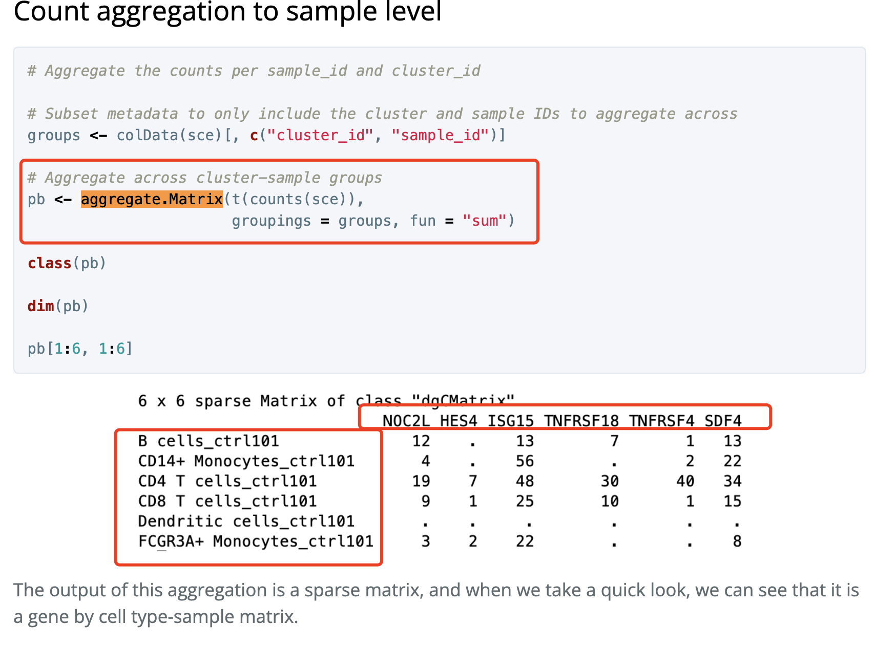
Matrix.utils包的aggregate.Matrix函数
这个是出自于 https://hbctraining.github.io/scRNA-seq/lessons/pseudobulk_DESeq2_scrnaseq.html
如下所示: