数据挖掘真的是把人逼到花样百出,我们《生信技能树》作为华语圈生物信息学自媒体界扛把子自然也是被各种开脑洞的思路“骚扰”着,不过大家请不要无限制的怼我的私人微信哈,如果提问,在公众号推文文末留言即可,或者发邮件给我,我的邮箱是 jmzeng1314@163.com
首先加载seurat数据集 , 这里就是pbmc3k 这个数据集举例子哈 :
library(SeuratData) #加载seurat数据集
getOption('timeout')
options(timeout=10000)
#InstallData("pbmc3k")
data("pbmc3k")
sce <- pbmc3k.final
table(Idents(sce))
然后可以单独拿出来表达量矩阵,并且查看基因情况,进行分成为编码和非编码。
ct=sce@assays$RNA@counts
ct[1:4,1:4]
dim(ct)
library(AnnoProbe)
ids=annoGene( rownames(ct),'SYMBOL','human')
head(ids)
tail(sort(table(ids$biotypes)))
lncGenes= unique(ids[ids$biotypes=='lncRNA',1])
pbGenes = unique(ids[ids$biotypes=='protein_coding',1])
可以看到,这个数据集里面的基因数量有点少:
#  13714 features across 2638 samples within 1 assay
                            lncRNA                     protein_coding
                               353                              11320
绝大部分都是 protein_coding,仅仅是353个lncRNA,基本上可以判定 10X这样的单细胞转录组里面的非编码基因信息很难挖掘了。
虽然lncRNA基因数量少,但是表达量占比还可以:
sce=PercentageFeatureSet(sce, features = lncGenes ,
col.name = "percent_lncGenes")
fivenum(sce@meta.data$percent_lncGenes)
C=sce@assays$RNA@counts
dim(C)
C=Matrix::t(Matrix::t(C)/Matrix::colSums(C)) * 100
# 这里的C 这个矩阵,有一点大,可以考虑随抽样
C=C[,sample(1:ncol(C),1000)]
boxplot(as.matrix(Matrix::t(C[lncGenes, ])),
cex = 0.1, las = 1,
xlab = "% total count per cell",
col = (scales::hue_pal())(50)[50:1],
horizontal = TRUE)
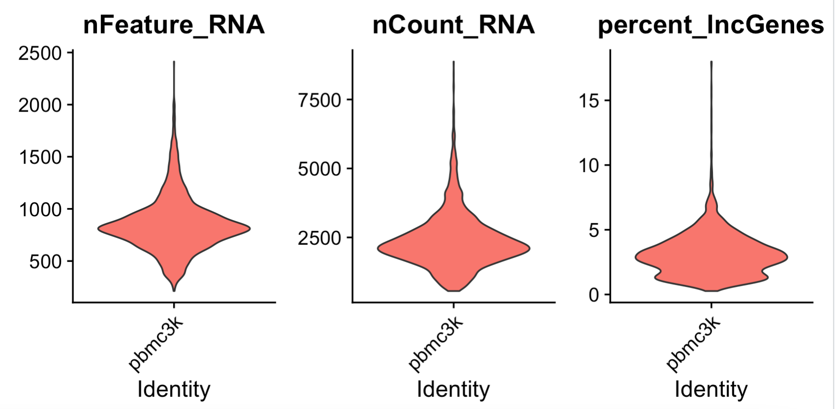
#可视化细胞的上述比例情况
feats <- c("nFeature_RNA", "nCount_RNA","percent_lncGenes")
p1=VlnPlot(sce, group.by = "orig.ident",
features = feats, pt.size = 0, ncol = 3) +
NoLegend()
p1
library(ggplot2)
ggsave(filename="Vlnplot1.pdf",plot=p1)
可以看到,跟绝大部分单细胞的线粒体基因百分比相当:
我们接下来分别对编码和非编码基因构成的独立矩阵进行降维聚类分群,看看效果。这样的单细胞转录组数据分析的标准降维聚类分群,并且进行生物学注释后的结果。可以参考前面的例子:人人都能学会的单细胞聚类分群注释 ,我们演示了第一层次的分群。如果你对单细胞数据分析还没有基础认知,可以看基础10讲:
代码如下所示:
首先是 蛋白质编码基因:
sce = CreateSeuratObject(
counts = ct[pbGenes,]
)
sce <- NormalizeData(sce)
sce <- FindVariableFeatures(sce )
sce <- ScaleData(sce )
sce <- RunPCA(sce, verbose = FALSE)
sce <- FindNeighbors(sce, dims = 1:10, verbose = FALSE)
sce <- FindClusters(sce, resolution = 0.5, verbose = FALSE)
sce <- RunUMAP(sce, dims = 1:10, umap.method = "uwot", metric = "cosine")
table(sce$seurat_clusters)
umap_pbGenes= DimPlot(sce,label = T,repel = T)
sce_pbGenes = sce
然后是非编码基因:
sce = CreateSeuratObject(
counts = ct[lncGenes,]
)
sce <- NormalizeData(sce)
sce <- FindVariableFeatures(sce )
sce <- ScaleData(sce )
sce <- RunPCA(sce, features = VariableFeatures(object = sce),
verbose = FALSE)
sce <- FindNeighbors(sce, dims = 1:10, verbose = FALSE)
sce <- FindClusters(sce, resolution = 0.5, verbose = FALSE)
sce <- RunUMAP(sce, dims = 1:10, umap.method = "uwot", metric = "cosine")
table(sce$seurat_clusters)
sce_lncGenes = sce
umap_lncGenes = DimPlot(sce,label = T,repel = T)
结合起来看看:
library(patchwork) umap_lncGenes + umap_pbGenes
可以看到右边的蛋白质编码基因矩阵的降维聚类分群没有问题:
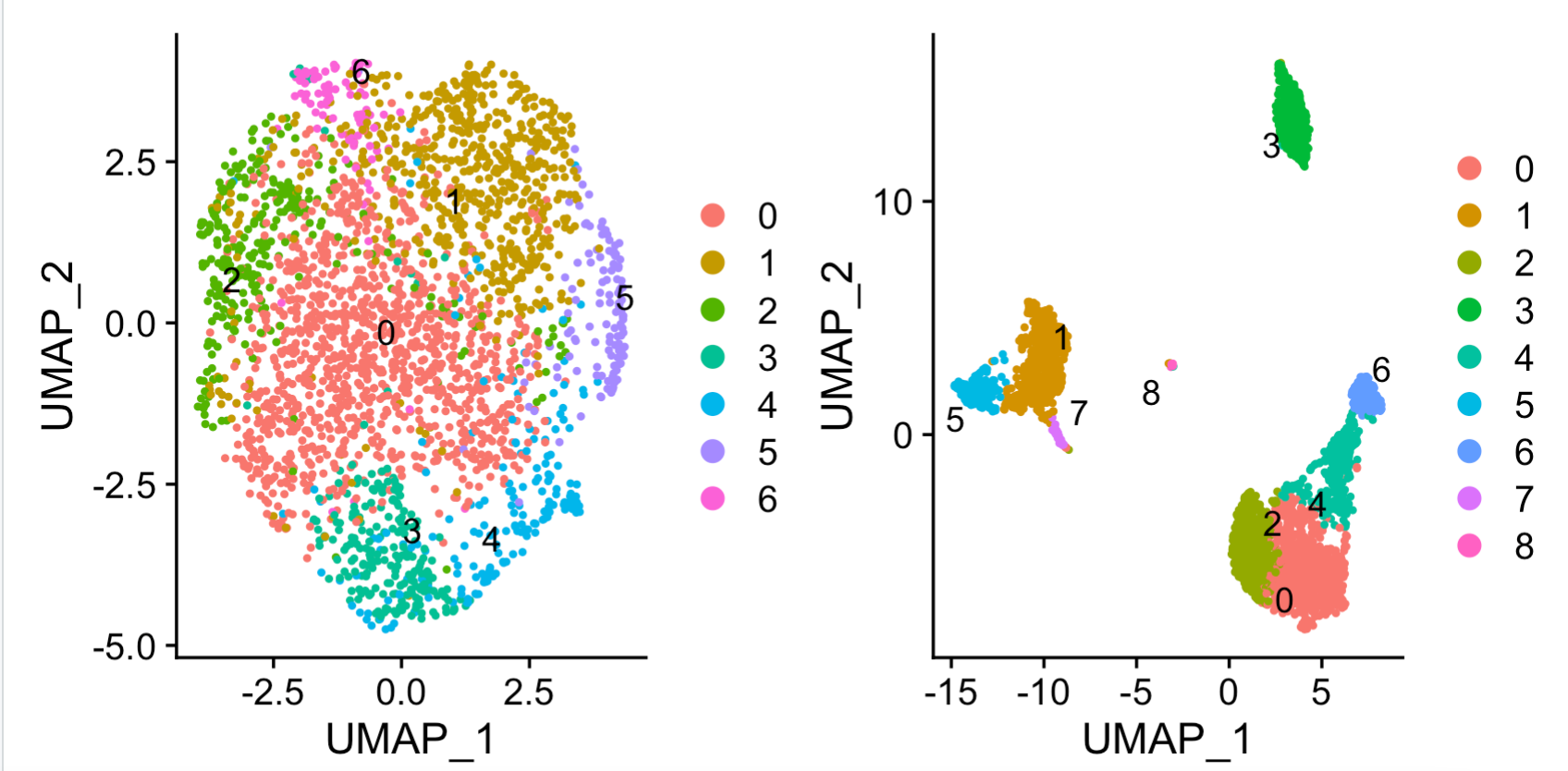
但是左边的非编码基因矩阵,走这个降维聚类分群基本上惨不忍睹。
然后具体看看两个分群的差异:
identical(colnames(sce_lncGenes),colnames(sce_pbGenes))
library(gplots)
balloonplot(table(
sce_lncGenes$seurat_clusters,
Idents(pbmc3k.final)
))
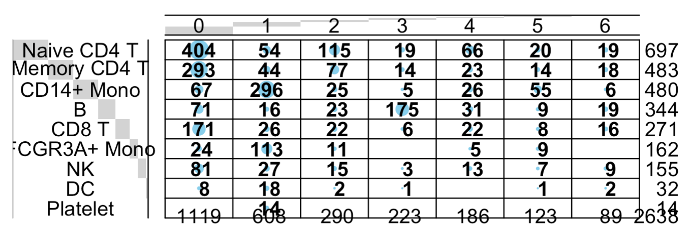
balloonplot(table(
sce_pbGenes$seurat_clusters,
Idents(pbmc3k.final)
))
也是同样的结论蛋白质编码基因矩阵的降维聚类分群基本上符合先验知识 ,
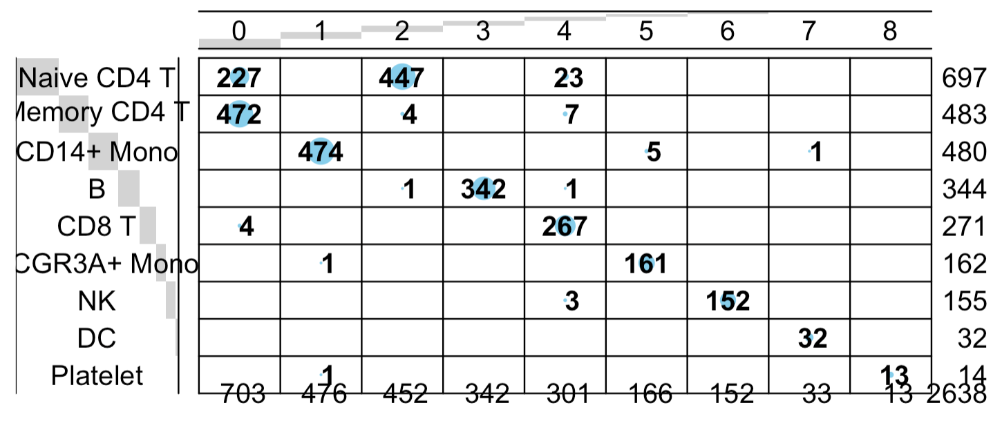
非编码的仍然是惨不忍睹:
如果是其它单细胞技术呢?
比如大名鼎鼎的smart-seq2,我相信结论肯定是不一样。
比如经典的 scRNAseq 这个 R包中的数据集,这个包内置的是 Pollen et al. 2014 数据集,人类单细胞细胞,分成4类,分别是 pluripotent stem cells 分化而成的 neural progenitor cells (“NPC”) ,还有 “GW16” and “GW21” ,“GW21+3” 这种孕期细胞,理解这些需要一定的生物学背景知识,如果不感兴趣,可以略过。
代码如下所示:
rm(list=ls())
options(stringsAsFactors = F)
library(Seurat)
# BiocManager::install('scRNAseq')
library(scRNAseq)
fluidigm <- ReprocessedFluidigmData()
fluidigm
ct <- floor(assays(fluidigm)$rsem_counts)
ct[1:4,1:4]
dim(ct)
ct=ct[rowSums(ct>1)>10,]
dim(ct)
ct[1:4,1:4]
dim(ct)
library(AnnoProbe)
ids=annoGene( rownames(ct),'SYMBOL','human')
head(ids)
tail(sort(table(ids$biotypes)))

lncGenes= unique(ids[ids$biotypes=='lncRNA',1])

sce = CreateSeuratObject(
  counts = ct[lncGenes,]
)
sce <- NormalizeData(sce)
sce <- FindVariableFeatures(sce )
sce <- ScaleData(sce )
sce <- RunPCA(sce, features = VariableFeatures(object = sce),
              verbose = FALSE)
sce <- FindNeighbors(sce, dims = 1:10, verbose = FALSE)
sce <- FindClusters(sce, resolution = 0.5, verbose = FALSE)
sce <- RunUMAP(sce, dims = 1:10, umap.method = "uwot", metric = "cosine")
table(sce$seurat_clusters)
sce_lncGenes = sce
umap_lncGenes = DimPlot(sce,label = T,repel = T)
umap_lncGenes

table(
  colData(fluidigm)$Biological_Condition,
  sce$seurat_clusters
)
蛮有意思的,这个数据集其实lncRNA数量也很少:
 lncRNA                     protein_coding
  278                               8965
但是它独立的降维聚类分群就看起来好很多:
          0  1
  GW16   42 10
  GW21   16  0
  GW21+3 31  1
  NPC     0 30
起码能够区分先验知识里面的 NPC和非NPC细胞。
写在文末
我在《生信技能树》,《生信菜鸟团》,《单细胞天地》的大量推文教程里面共享的代码都是复制粘贴即可使用的, 有任何疑问欢迎留言讨论,也可以发邮件给我,详细描述你遇到的困难的前因后果给我,我的邮箱地址是 jmzeng1314@163.com
如果你确实觉得我的教程对你的科研课题有帮助,让你茅塞顿开,或者说你的课题大量使用我的技能,烦请日后在发表自己的成果的时候,加上一个简短的致谢,如下所示:
We thank Dr.Jianming Zeng(University of Macau), and all the members of his bioinformatics team, biotrainee, for generously sharing their experience and codes.
十年后我环游世界各地的高校以及科研院所(当然包括中国大陆)的时候,如果有这样的情谊,我会优先见你。