背景介绍:
DNA 甲基化是一种表观遗传标记,可限制染色质的可及性,并在器官发生过程中调节时空基因表达。Dnmt1 是研究最多的 DNA 甲基转移酶之一,它主要参与保存进行有丝分裂的细胞中的 DNA 甲基化模式。其中Dnmt1 在胚胎肺内胚层中的作用已被发现,但其在胚胎肺中胚层的扩张、维持和分化中的作用还未见报道。GSE175640单细胞数据集,表明 Dnmt1 是胚胎肺中胚层正常发育至关重要。敲除胚胎肺中胚层中的 Dnmt1,发现 Dnmt1 严重影响胚胎脉管系统的发育和中胚层对肺间充质细胞谱系。
结果:
E7.5 期胚胎肺间质中的 Dnmt1 缺失导致致死表型,其特征是双侧肺发育不全、肺分支形态发生受损和实质广泛出血。
出血的起因可能是肺脉管系统发育停止,特别是在突变肺中检测到的周细胞个体发育。严重的间充质改变,肺内胚层的分化是正常的。当 Dnmt1 在发育后期 (E13.5) 被敲除时,肺正常成熟,突变体幼崽是有活力的,尽管在所有突变体动物出生后 7 天就观察到 Pdgfr-α 肌成纤维细胞的分化减少和肺泡简化。基因表达谱研究表明,Dnmt1 的缺失诱导了睾丸、胎盘和卵巢特异性基因的异位表达,如 Tex10.1、Tex19.1 和 Pet2,这表明肺中胚层对肺细胞谱系的功能丧失.
补充知识:pericyte 周细胞 又称外膜细胞,外皮细胞,周皮细胞:一种特殊的能收缩的长细胞,见于前毛细血管小动脉周围包绕基底膜处
结论:
综上所述,数据集研究结果表明,Dnmt1 在发育中的肺间充质中的表达对于限制肺中胚层的分化能力至关重要,从而确保胎儿和出生后肺中血管系统细胞和肌成纤维细胞的充分分化。
数据分析:
此次数据来源于NCBI数据库https://www.ncbi.nlm.nih.gov/geo/query/acc.cgi?acc=GSE175640
其中Wildtype 为野生型样本,Dnmt1 CKO为 Dnmt1 基因敲除样本,实验材料为小鼠。

存放在data目录下:

1. 数据读入
samples=list.files('../data/')
samples
sceList = lapply(samples,function(pro){
 # pro=samples[1]
 folder=file.path('../data',pro)
 print(pro)
 print(folder)
 print(list.files(folder))
 sce=CreateSeuratObject(counts = Read10X(folder),
 project = pro )

 return(sce)
})
names(sceList) = samples
sce.all <- merge(sceList[[1]], y= sceList[ -1 ] ,
 add.cell.ids=samples)
sce.all$group <- ifelse(sce.all$orig.ident %in% c("Wildtype_1","Wildtype_1"),"WT","DnCKO")
save(sce.all,file = "../subdata/sce.all.Rdata")
2. 数据质控过滤
# 质控和过滤 -------------------------------------------------------------------
#计算线粒体基因比例
# 人和鼠的基因名字稍微不一样
mito_genes=rownames(sce.all)[grep("^mt-", rownames(sce.all))]
mito_genes #13个线粒体基因
sce.all=PercentageFeatureSet(sce.all, "^mt-", col.name = "percent_mito")
fivenum(sce.all@meta.data$percent_mito)
#计算核糖体基因比例
ribo_genes=rownames(sce.all)[grep("^Rp[sl]", rownames(sce.all),ignore.case = T)]
ribo_genes
sce.all=PercentageFeatureSet(sce.all, "^Rp[sl]", col.name = "percent_ribo")
fivenum(sce.all@meta.data$percent_ribo)
#计算红血细胞基因比例
hb_genes <- rownames(sce.all)[grep("^Hb[^(p)]", rownames(sce.all),ignore.case = T)]
hb_genes
sce.all=PercentageFeatureSet(sce.all, "^Hb[^(p)]", col.name = "percent_hb")
fivenum(sce.all@meta.data$percent_hb)

selected_c <- WhichCells(sce.all, expression = nFeature_RNA >300) # 每个细胞中基因表达>300
selected_f <- rownames(sce.all)[Matrix::rowSums(sce.all@assays$RNA@counts > 0 ) > 3] # 至少在3个细胞中表达
sce.all.filt <- subset(sce.all, features = selected_f, cells = selected_c)
selected_mito <- WhichCells(sce.all.filt, expression = percent_mito < 15)
selected_ribo <- WhichCells(sce.all.filt, expression = percent_ribo > 3)
selected_hb <- WhichCells(sce.all.filt, expression = percent_hb < 0.1)
table(sce.all$orig.ident)
# DnCKO_1 DnCKO_2 Wildtype_1 Wildtype_2
# 7013 7820 6698 6284
table(sce.all.filt$orig.ident)
# DnCKO_1 DnCKO_2 Wildtype_1 Wildtype_2
# 1838 3004 3864 3787
3.降维聚类分群-检查批次效应
#数据预处理
sce<-sce.all.filt
sce <- NormalizeData(sce)
sce = ScaleData(sce,
features = rownames(sce),
# vars.to.regress = c("nFeature_RNA", "percent_mito")
) #加上vars.to.regress参数后运行so slow!!!
# 降维处理
sce <- FindVariableFeatures(sce, nfeatures = 3000)
set.seed(175640)
sce <- RunPCA(sce, npcs = 30)
sce <- RunTSNE(sce, dims = 1:30)
sce <- RunUMAP(sce, dims = 1:30)
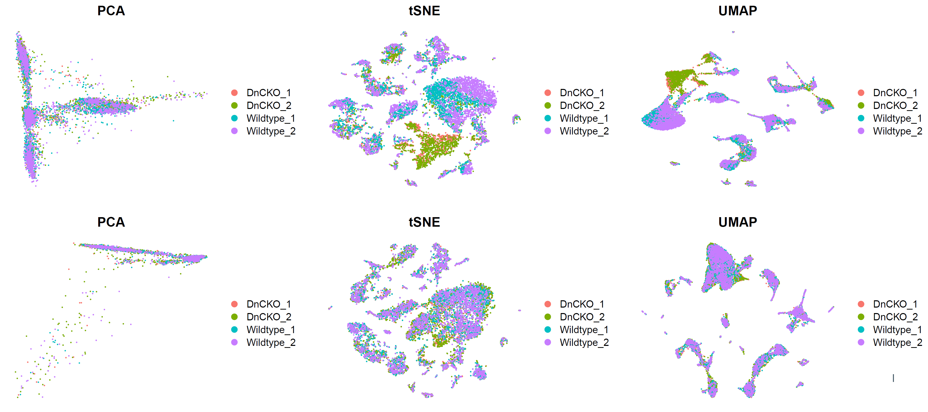
# 检查批次效应 ------------------------------------------------------------------
colnames(sce@meta.data)
# [1] "orig.ident" "nCount_RNA" "nFeature_RNA"
# [4] "percent_mito" "percent_ribo" "percent_hb"
p1.compare=plot_grid(ncol = 3,
DimPlot(sce, reduction = "pca", group.by = "orig.ident")+NoAxes()+ggtitle("PCA"),
DimPlot(sce, reduction = "tsne", group.by = "orig.ident")+NoAxes()+ggtitle("tSNE"),
DimPlot(sce, reduction = "umap", group.by = "orig.ident")+NoAxes()+ggtitle("UMAP")
)
p1.compare
ggsave(plot=p1.compare,filename="../picture/2_PCA_UMAP_TSNE/Before_inter_1.pdf")
DimPlot(sce,
reduction = "umap", # pca, umap, tsne
group.by = "orig.ident",
label = F)
ggsave("../picture/2_PCA_UMAP_TSNE/Dimplot_before_1.pdf",units = "cm", width = 20,height = 18)
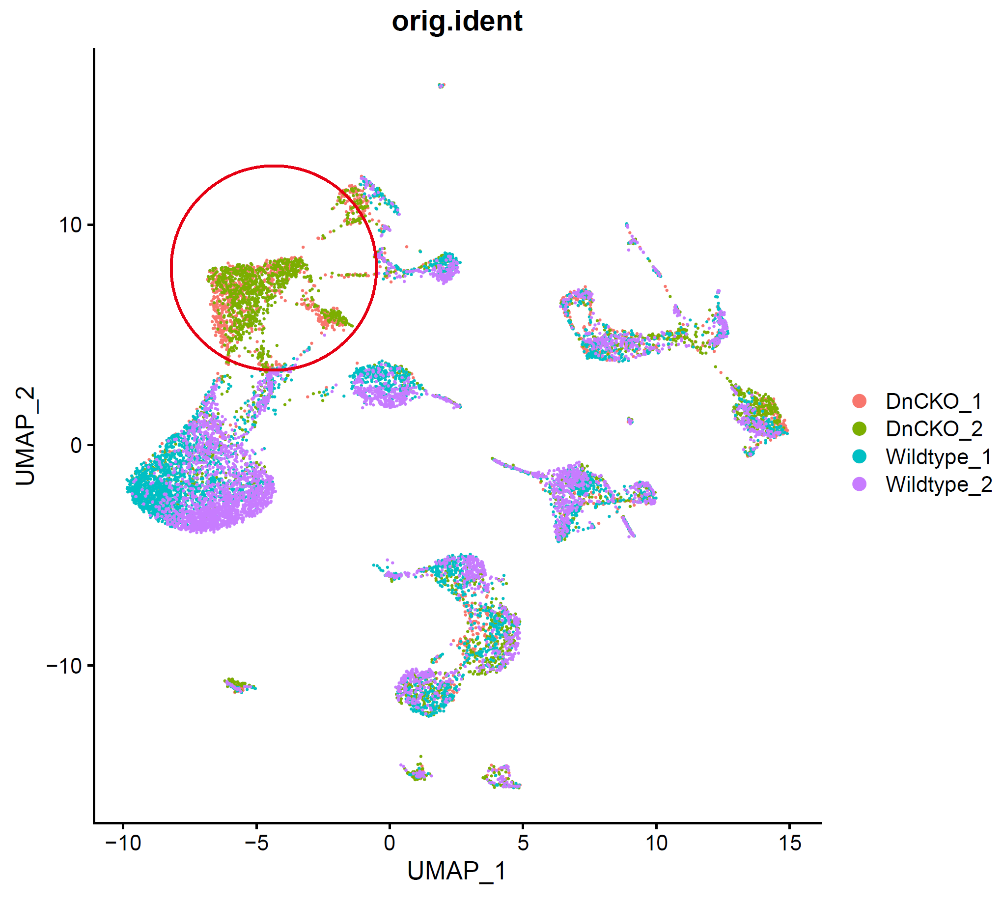
存在明显的样本特异性,需要去除批次效应,降低样本间差异。
4. 去除批次效应—CCA
# CCA 去除批次效应 --------------------------------------------------------------
sce.all=sce
sce.all
# An object of class Seurat
# 21754 features across 40222 samples within 1 assay
# Active assay: RNA (21754 features, 3000 variable features)
# 3 dimensional reductions calculated: pca, tsne, umap

#拆分为 个seurat子对象
sce.all.list <- SplitObject(sce.all, split.by = "orig.ident")
sce.all.list
for (i in 1:length(sce.all.list)) {
 print(i)
 sce.all.list[[i]] <- NormalizeData(sce.all.list[[i]], verbose = FALSE)
 sce.all.list[[i]] <- FindVariableFeatures(sce.all.list[[i]], selection.method = "vst",
 nfeatures = 2000, verbose = FALSE)
}
#耗时,1h~2h左右
alldata.anchors <- FindIntegrationAnchors(object.list = sce.all.list, dims = 1:30,
 reduction = "cca")
sce.all.int <- IntegrateData(anchorset = alldata.anchors, dims = 1:30, new.assay.name = "CCA")
names(sce.all.int@assays)
#[1] "RNA" "CCA"
sce.all.int@active.assay
#[1] "CCA"
sce.all.int=ScaleData(sce.all.int)
sce.all.int=RunPCA(sce.all.int, npcs = 30)
sce.all.int=RunTSNE(sce.all.int, dims = 1:30)
sce.all.int=RunUMAP(sce.all.int, dims = 1:30)
names(sce.all.int@reductions)
# 检查批次效应----
p2.compare=plot_grid(ncol = 3,
 DimPlot(sce.all.int, reduction = "pca", group.by ="orig.ident")+NoAxes()+ggtitle("PCA"),
 DimPlot(sce.all.int, reduction = "tsne", group.by="orig.ident")+NoAxes()+ggtitle("tSNE"),
 DimPlot(sce.all.int, reduction = "umap", group.by = "orig.ident")+NoAxes()+ggtitle("UMAP")
)
p2.compare
ggsave(plot=p2.compare,filename="../picture/2_PCA_UMAP_TSNE/Before_inter_CCA_2.pdf",units = "cm",width = 27,height = 8)
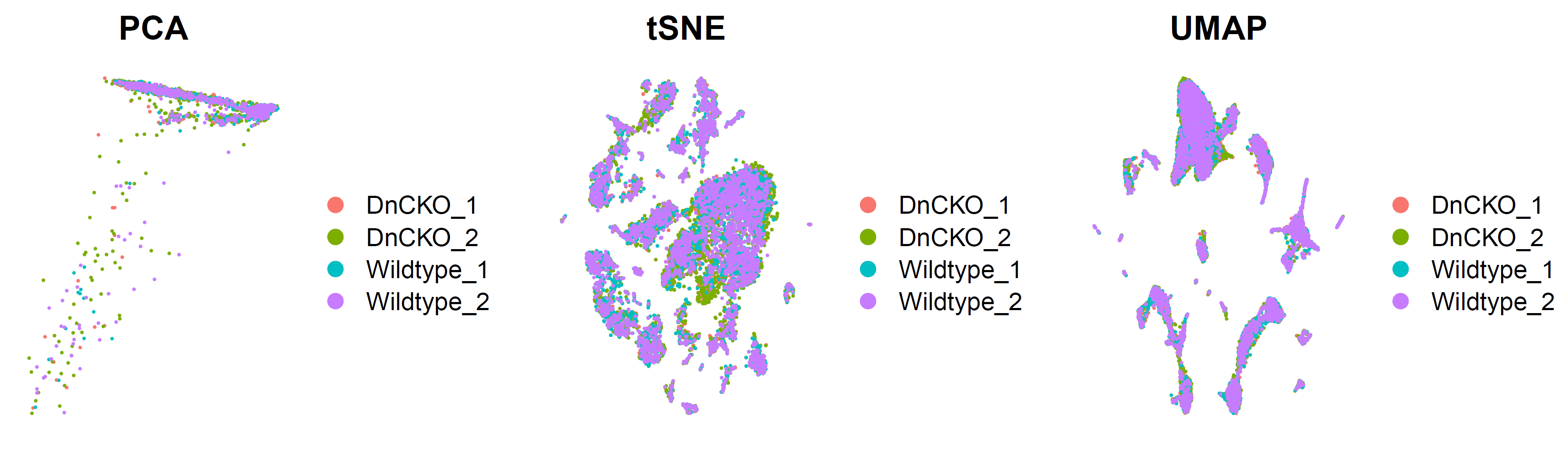
去除批次效应前后对比:
# CCA 比较去除批次前后 --------------------------------------------------------
p5.compare=plot_grid(ncol = 3,
 DimPlot(sce, reduction = "pca", group.by = "orig.ident")+NoAxes()+ggtitle("PCA"),
 DimPlot(sce, reduction = "tsne", group.by = "orig.ident")+NoAxes()+ggtitle("tSNE"),
 DimPlot(sce, reduction = "umap", group.by = "orig.ident")+NoAxes()+ggtitle("UMAP"),

 DimPlot(sce.all.int, reduction = "pca", group.by = "orig.ident")+NoAxes()+ggtitle("PCA"),
 DimPlot(sce.all.int, reduction = "tsne", group.by = "orig.ident")+NoAxes()+ggtitle("tSNE"),
 DimPlot(sce.all.int, reduction = "umap", group.by = "orig.ident")+NoAxes()+ggtitle("UMAP")
)
p5.compare
ggsave(plot=p5.compare,filename="../picture/2_PCA_UMAP_TSNE/umap_by_har_before_after.pdf",units = "cm", width = 40,height = 18)
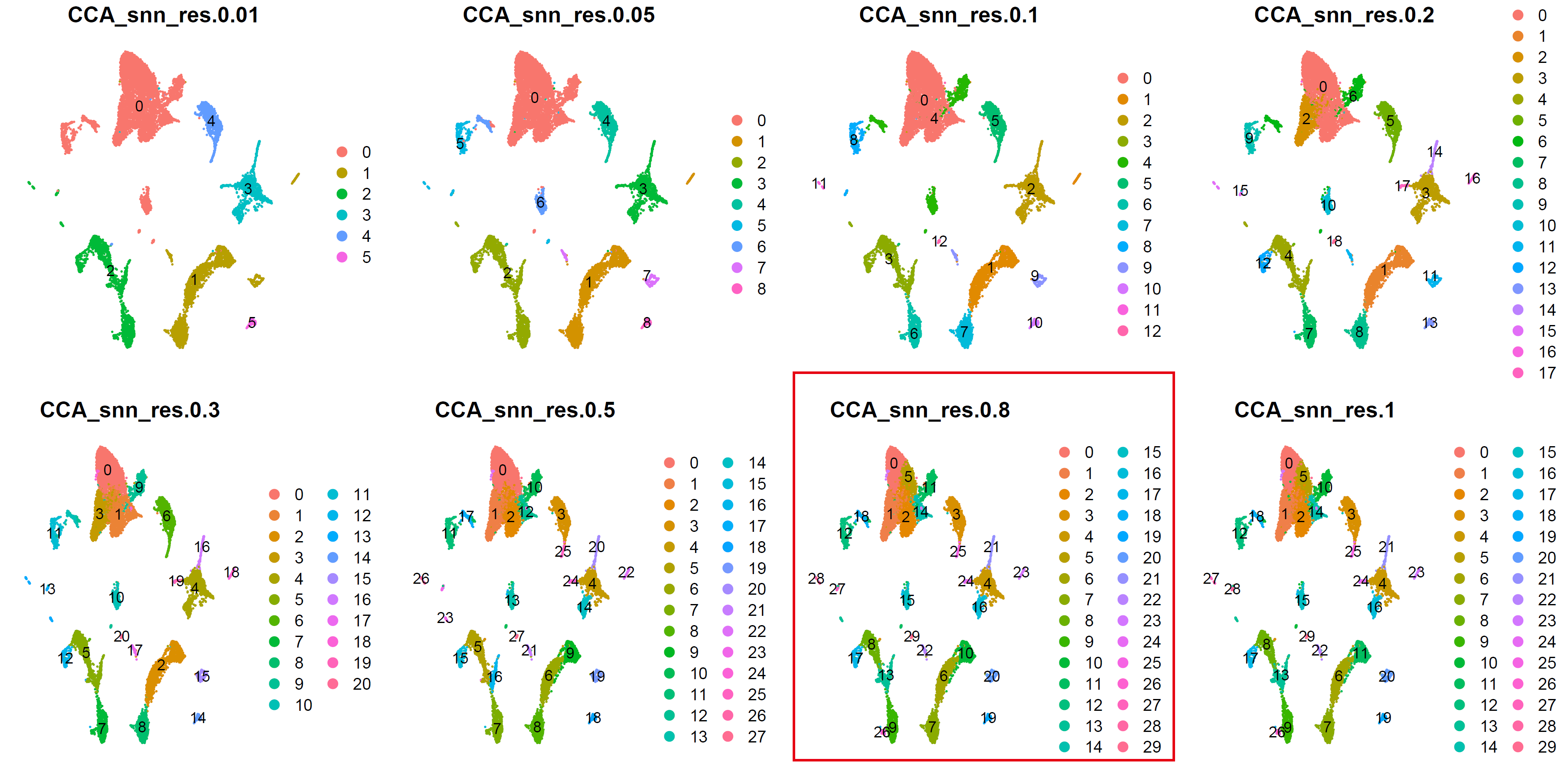
细胞分群:
sce <- sce.all.int
sce <- FindNeighbors(sce, dims = 1:30)
for (res in c(0.01, 0.05, 0.1, 0.2, 0.3, 0.5,0.8,1)) {
 # res=0.01
 print(res)
 sce <- FindClusters(sce, graph.name = "CCA_snn", resolution = res, algorithm = 1)
}
#umap可视化
cluster_umap <- plot_grid(ncol = 4,
 DimPlot(sce, reduction = "umap", group.by = "CCA_snn_res.0.01", label = T) & NoAxes(),
 DimPlot(sce, reduction = "umap", group.by = "CCA_snn_res.0.05", label = T)& NoAxes(),
 DimPlot(sce, reduction = "umap", group.by = "CCA_snn_res.0.1", label = T) & NoAxes(),
 DimPlot(sce, reduction = "umap", group.by = "CCA_snn_res.0.2", label = T)& NoAxes(),
 DimPlot(sce, reduction = "umap", group.by = "CCA_snn_res.0.3", label = T)& NoAxes(),
 DimPlot(sce, reduction = "umap", group.by = "CCA_snn_res.0.5", label = T) & NoAxes(),
 DimPlot(sce, reduction = "umap", group.by = "CCA_snn_res.0.8", label = T) & NoAxes(),
 DimPlot(sce, reduction = "umap", group.by = "CCA_snn_res.1", label = T) & NoAxes()
)
cluster_umap
ggsave(cluster_umap, filename = "../picture/2_PCA_UMAP_TSNE/cluster_umap_all_res_by_CCA.pdf", width = 16, height = 8)
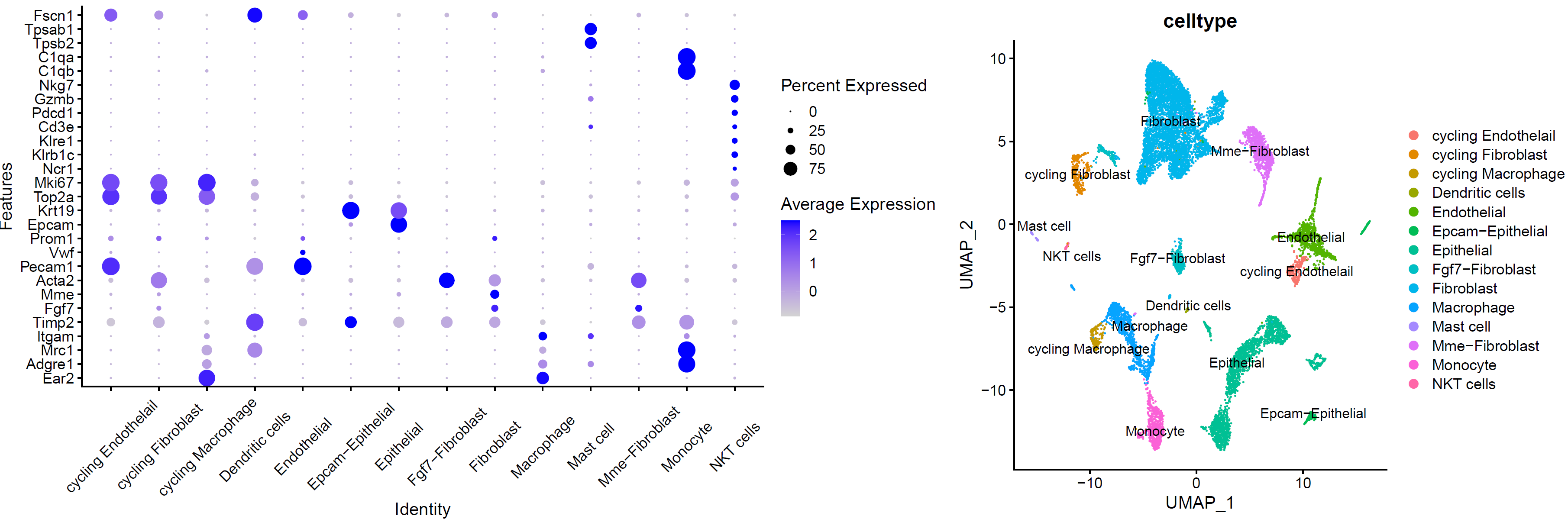
5. 细胞亚群注释
# 注释细胞亚群 ------------------------------------------------------------------
###### step6: 细胞类型注释 (根据marker gene) ######
celltype=data.frame(ClusterID=0:29,
 celltype='NA')
celltype[celltype$ClusterID %in% c( 8,13,9),2]='Macrophage' # "Ear2","Adgre1"."Mrc1","Itgam","Timp2"
celltype[celltype$ClusterID %in% c( 0,1,2,5,14,11,18 ),2]='Fibroblast' # "Fgf7","Mme","Acta2"
celltype[celltype$ClusterID %in% c( 4,24,21 ),2]='Endothelial' # "Pecam1","Vwf","Prom1"
celltype[celltype$ClusterID %in% c( 6,7,10,22,20 ),2]='Epithelial' # "Epcam","Krt19"
celltype[celltype$ClusterID %in% c( 12 ),2]='cycling Fibroblast'
celltype[celltype$ClusterID %in% c( 16 ),2]='cycling Endothelail' #"Top2a","Mki67"
celltype[celltype$ClusterID %in% c(27 ),2]='NKT cells' # "Ncr1","Klrb1c","Klre1","Cd3e","Pdcd1","Gzmb"
celltype[celltype$ClusterID %in% c(9, 26 ),2]='Monocyte' # "C1qb","C1qa"
celltype[celltype$ClusterID %in% c( 17 ),2]='cycling Macrophage'
celltype[celltype$ClusterID %in% c( 28 ),2]='Mast cell' # "Tpsb2","Tpsab1"
celltype[celltype$ClusterID %in% c( 3,25 ),2]='Mme-Fibroblast'
celltype[celltype$ClusterID %in% c( 29),2]='Dendritic cells' # "Fscn1"
celltype[celltype$ClusterID %in% c( 19,23 ),2]='Epcam-Epithelial'
celltype[celltype$ClusterID %in% c( 15,18 ),2]='Fgf7-Fibroblast'
head(celltype)
celltype
table(celltype$celltype)
sce.all@meta.data$celltype = "NA"
for(i in 1:nrow(celltype)){
 sce.all@meta.data[which(sce.all@meta.data$CCA_snn_res.0.8 == celltype$ClusterID[i]),'celltype'] <- celltype$celltype[i]}
table(sce.all@meta.data$celltype)
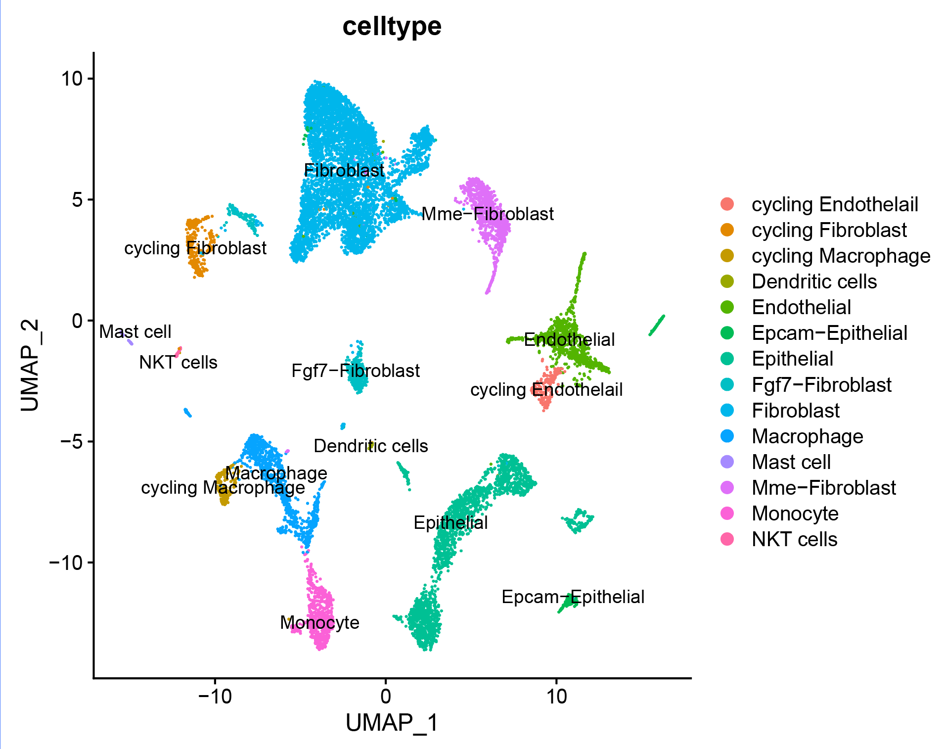
注释结果可视化:
# umap_by_celltype --------------------------------------------------------
th=theme(axis.text.x = element_text(angle = 45,
 vjust = 0.5, hjust=0.5))
genes_to_check <- c("Ear2","Adgre1","Mrc1","Itgam","Timp2","Fgf7","Mme","Acta2","Pecam1","Vwf","Prom1","Epcam","Krt19", "Top2a","Mki67","Ncr1","Klrb1c","Klre1","Cd3e","Pdcd1","Gzmb","Nkg7","C1qb","C1qa","Tpsb2","Tpsab1","Fscn1")
p_all_markers=DotPlot(sce.all, features = genes_to_check,
 group.by = "celltype",assay='RNA' ) + coord_flip()+th

color <- c('#e41a1c','#377eb8','#4daf4a','#984ea3','#ff7f00','#ffff33','#a65628','#f781bf','#999999')
p_umap<- DimPlot(sce.all, reduction = "umap", group.by = "celltype",label = T)
p_umap
ps <- plot_grid(p_all_markers,p_umap,rel_widths = c(1.5,1))
ps
ggsave(ps,filename = "../picture/Annotation/our_markers_dotplot_by_celltype.pdf",units = "cm",width = 60,height = 30)

p_celltype<- DimPlot(sce.all, reduction = "tsne",group.by = "celltype",label = T)
p_celltype
ggsave(p_celltype,filename = '../picture/Annotation/tsne_by_celltype.pdf',width = 20,height = 16,units = "cm")

p_celltype<- DimPlot(sce.all, reduction = "umap",group.by = "celltype",label = T)
p_celltype
ggsave(p_celltype,filename = '../picture/Annotation/umap_by_celltype.pdf',width = 20,height = 16,units = "cm")
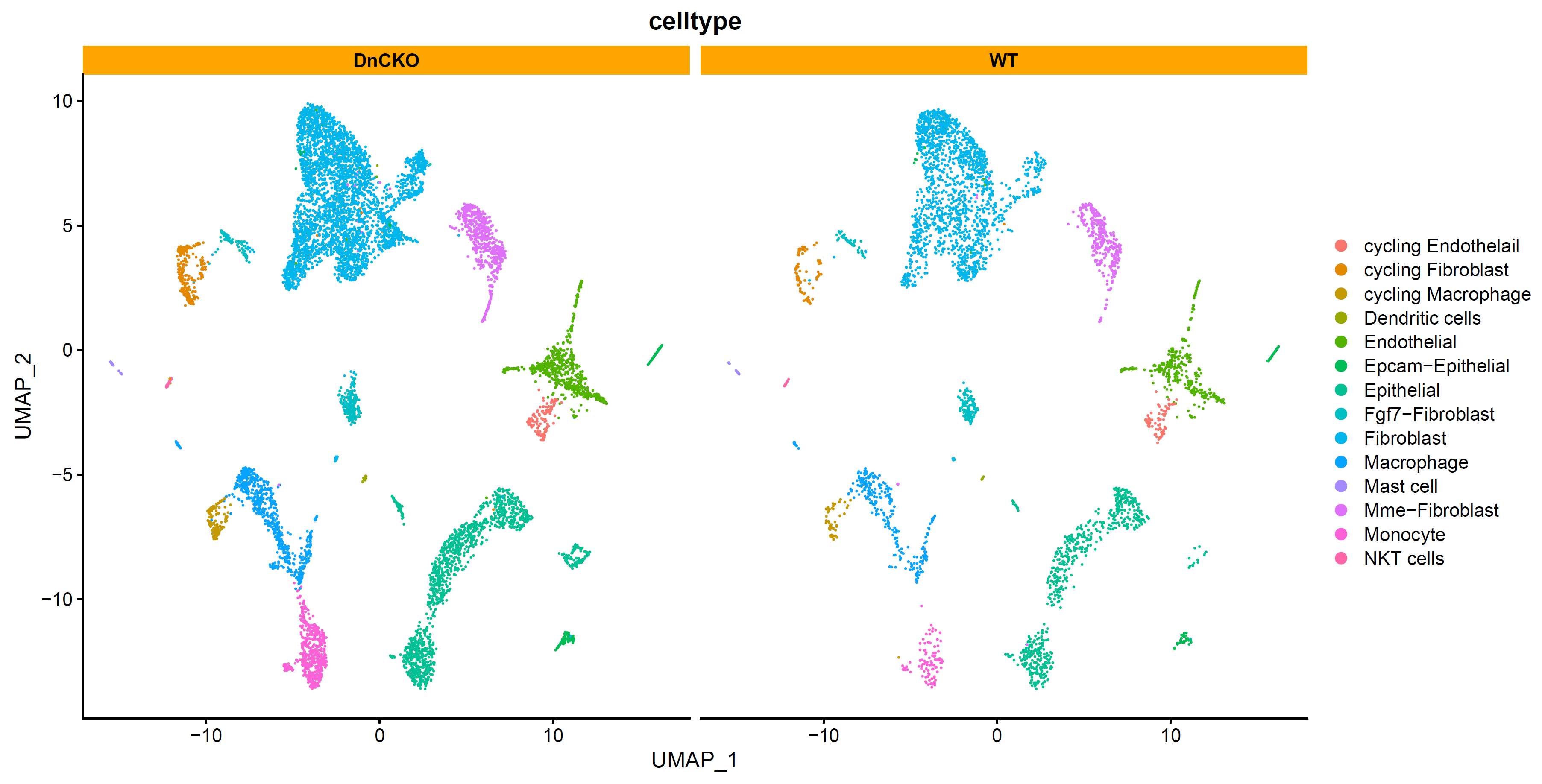
查看细胞分布:
# split by group ----
p4 <- DimPlot(sce.all, reduction = "umap", group.by = "celltype",split.by = "group",label = F,label.size = 6)+facet_wrap(~group)+theme(strip.background = element_rect(fill="orange"))
p4
ggsave(p4,filename = "../picture/Annotation/umap_by_group_celltype.pdf",units = "cm",width = 35,height = 18)
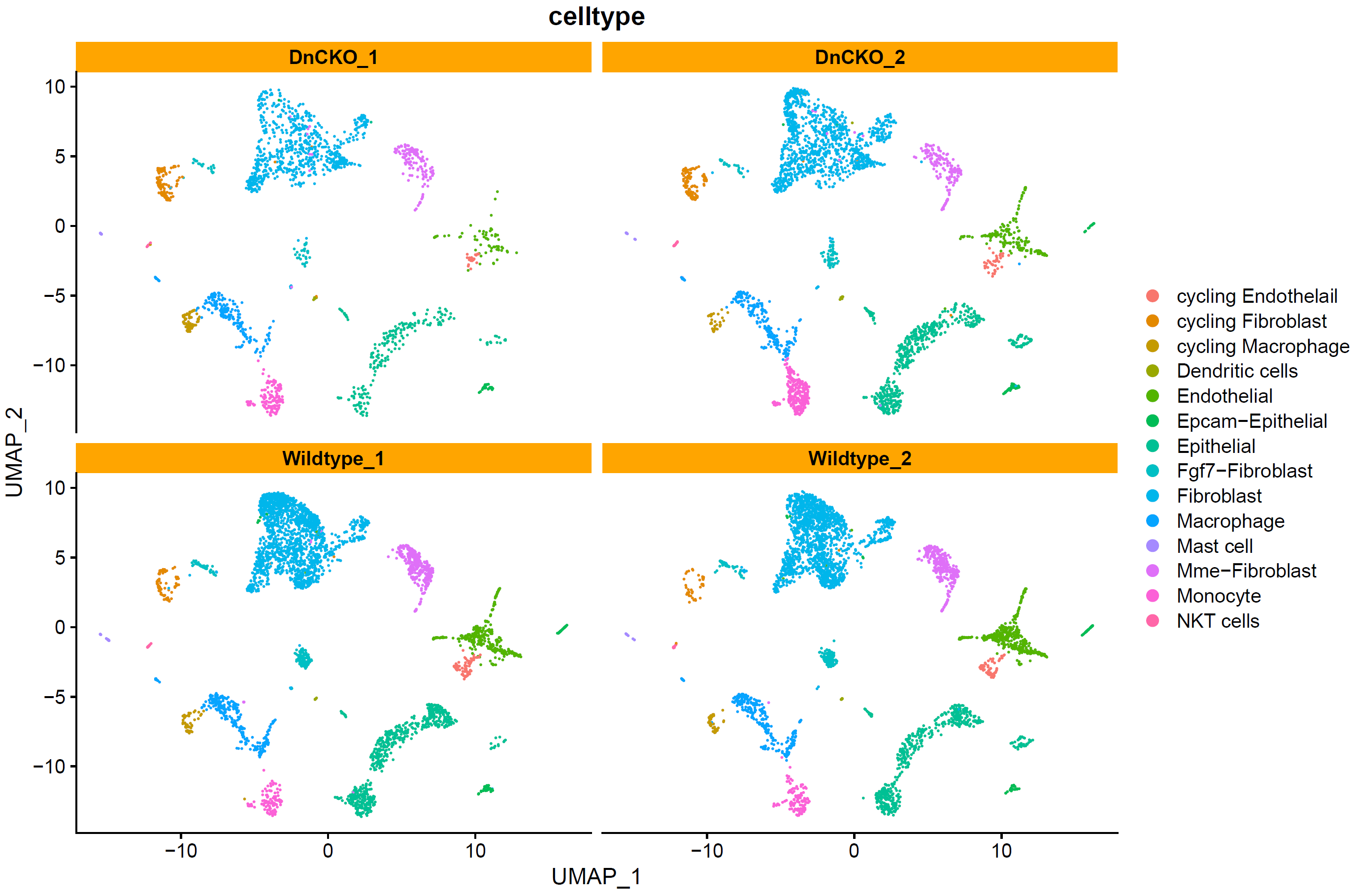
# split by orig.ident ----
p5 <- DimPlot(sce.all, reduction = "umap", group.by = "celltype",split.by = "orig.ident",label = F)+
facet_wrap(~orig.ident)+theme(strip.background = element_rect(fill="orange"))
p5
ggsave(p5,filename = "../picture/Annotation/umap_by_orig.ident_celltype.pdf",units = "cm",width = 30,height = 20)
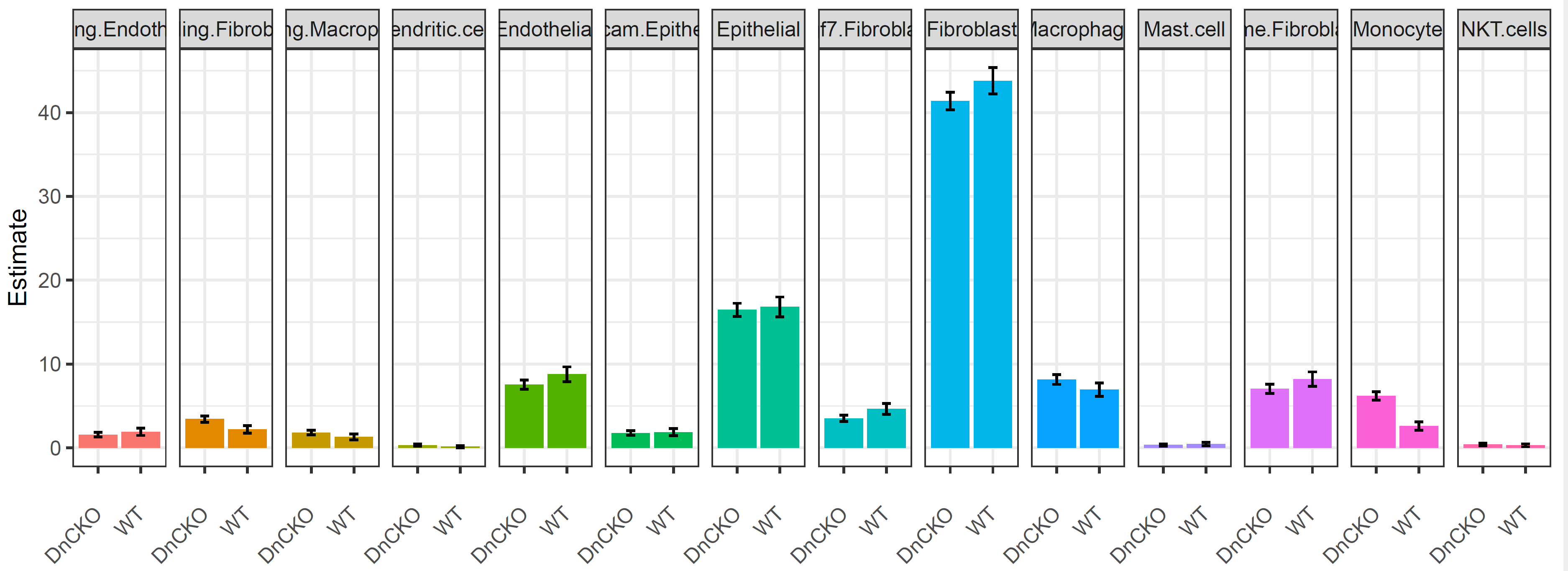
细胞比例变化:
head(phe)
if(T){
 library(ggrepel)
 require(qdapTools)
 require(REdaS)
 metadata <- phe
 meta.temp <- metadata[,c( "group","celltype")]
 colnames(meta.temp)=c("analysis","immuSub")
 write.csv(phe,file = "../subdata/phe.csv")
 # Loop over treatment response categories
 # Create list to store frequency tables
 prop.table.error <- list()
 for(i in 1:length(unique(meta.temp$analysis))){
 vec.temp <- meta.temp[meta.temp$analysis==unique(meta.temp$analysis)[i],"immuSub"]
 # Convert to counts and calculate 95% CI
 # Store in list
 table.temp <- freqCI(vec.temp, level = c(.95))
 prop.table.error[[i]] <- print(table.temp, percent = TRUE, digits = 3)
 #
 }
 # Name list
 names(prop.table.error) <- unique(meta.temp$analysis)
 # Convert to data frame
 tab.1 <- as.data.frame.array(do.call(rbind, prop.table.error))
 # Add analysis column
 b <- c()
 a <- c()
 for(i in names(prop.table.error)){
 a <- rep(i,nrow(prop.table.error[[1]]))
 b <- c(b,a)
 }
 tab.1$analysis <- b
 # Add common cell names
 aa <- gsub(x = row.names(tab.1), ".1", "")
 tab.1$cell <- aa
 write.csv(tab.1,file = "Realtive_subcluster_input_data.csv")
 # Resort factor analysis
 # Rename percentile columns
 colnames(tab.1)[1] <- "lower"
 colnames(tab.1)[3] <- "upper"
 p<- ggplot(tab.1, aes(x=analysis, y=Estimate, group=cell)) +
 geom_line(aes(color=cell))+
 geom_point(aes(color=cell)) + facet_grid(cols = vars(cell)) +
 theme(axis.text.x = element_text(angle = 45, hjust=1, vjust=0.5), legend.position="bottom") +
 xlab("") +
 geom_errorbar(aes(ymin=lower, ymax=upper), width=.2,position=position_dodge(0.05))
 p1<- ggplot(tab.1, aes(x=analysis, y=Estimate, group=cell)) +
 geom_bar(stat = "identity", aes(fill=cell)) + facet_grid(cols = vars(cell)) +
 theme_bw() +
 theme(axis.text.x = element_text(angle = 45, hjust=1, vjust=0.5), legend.position= "none") +
 xlab("") +
 geom_errorbar(aes(ymin=lower, ymax=upper), width=.2,position=position_dodge(0.05))
 p1
}
ggsave(p1,filename = "../picture/DEG/Realtive_subcluster.pdf",units = "cm",width = 24,height = 9)
哈哈,最终完成分析。