前面我们的泛癌系列教程,都是直接使用count矩阵进行分析,最多就是进行一些转换而已。但是很多读者不依不饶一定要我们使用TPM表达量矩阵,因为这个更权威或者说更流行!
首先需要下载TCGA的33种癌症的全部数据,尤其是表达量矩阵和临床表型信息啦,这里我们推荐在ucsc的xena里面下载:https://xenabrowser.net/datapages/,可以看到,确实是没有提供TPM表达量矩阵,但是自己进行转换啊!无论RPKM或FPKM或者TPM格式是多么的遭人诟病,它的真实需求还是存在, 那么我们该如何合理的定义基因的长度呢?
这个时候需要理解:基因,转录本(transcripts,isoform,mRNA序列)、EXON区域,cDNA序列、UTR区域,ORF序列、CDS序列 这些概念,一个基因可以转录为多个转录本,真核生物里面每个转录本通常是由一个或者多个EXON组成,能翻译为蛋白的EXON区域是CDS区域,不能翻译的那些EXON的开头和结尾是UTR区域,翻译区域合起来是ORF序列,而转录本逆转录就是cDNA序列。
关于基因长度的探讨
五年前我分享过前主流定义基因长度的几种方式。
- 挑选基因的最长转录本
- 选取多个转录本长度的平均值
- 非冗余外显子(EXON)长度之和
- 非冗余 CDS(Coding DNA Sequence) 长度之和
参考我的博客:定义基因长度为非冗余CDS之和 http://www.bio-info-trainee.com/3298.html
其它参考举例:
- https://www.uniprot.org/uniprot/A2CE44
- http://www.informatics.jax.org/marker/MGI:3694898
- http://www.informatics.jax.org/sequence/marker/MGI:3694898?provider=RefSeq
- https://asia.ensembl.org/Mus_musculus/Gene/Summary?g=ENSMUSG00000073062
- https://www.ncbi.nlm.nih.gov/CCDS/CcdsBrowse.cgi?REQUEST=CCDS&DATA=CCDS41065.1
CCDS文件里面:
X NC_000086.7 Zxdb 668166 CCDS41065.1 Public + 94724674 94727295 [94724674-94727295] Identical
可以看到不同的定义,得到的基因长度定义还是差异很大的。
我这里有一个代码可以获取小鼠的 基因长度,基于 非冗余exon长度之和:
# BiocManager::install('TxDb.Hsapiens.UCSC.hg38.knownGene')
library("TxDb.Hsapiens.UCSC.hg38.knownGene")
txdb <- TxDb.Hsapiens.UCSC.hg38.knownGene

## 下面是定义基因长度为 非冗余exon长度之和
if(!file.exists('gene_length.Rdata')){
 exon_txdb=exons(txdb)
 genes_txdb=genes(txdb)

 o = findOverlaps(exon_txdb,genes_txdb)
 o
 t1=exon_txdb[queryHits(o)]
 t2=genes_txdb[subjectHits(o)]
 t1=as.data.frame(t1)
 t1$geneid=mcols(t2)[,1]

 # 如果觉得速度不够,就参考R语言实现并行计算
 # http://www.bio-info-trainee.com/956.html
 g_l = lapply(split(t1,t1$geneid),function(x){
 # x=split(t1,t1$geneid)[[1]]
 head(x)
 tmp=apply(x,1,function(y){
 y[2]:y[3]
 })
 length(unique(unlist(tmp)))
 })
 head(g_l)
 g_l=data.frame(gene_id=names(g_l),length=as.numeric(g_l))

 save(g_l,file = 'gene_length.Rdata')
}

load(file = 'gene_length.Rdata')
head(g_l)
# 如果是需要其它物种, 换一个包就好了哈!
if(F){
 # BiocManager::install('TxDb.Mmusculus.UCSC.mm10.knownGene')
 library("TxDb.Mmusculus.UCSC.mm10.knownGene")
 txdb <- TxDb.Mmusculus.UCSC.mm10.knownGene


}
有了基因长度信息,就很容易转换啦!
首先检查表达量矩阵额基因长度信息:
> load(file = 'gene_length.Rdata')
> head(g_l)
 gene_id length
1 1 9488
2 10 1285
3 100 2809
4 1000 9054
5 10000 13977
6 100009613 1004
> load('../expression/Rdata/TCGA-ACC.htseq_counts.Rdata')
# 如果你不知道 TCGA-ACC.htseq_counts.Rdata 文件,去看前面的系列教程哦!
> pd_mat[1:4,1:4]
 TCGA-OR-A5JP-01A TCGA-OR-A5JG-01A TCGA-OR-A5K1-01A TCGA-OR-A5JR-01A
ZZZ3 1687 1583 784 1555
ZZEF1 1955 2036 697 2191
ZYX 2528 4567 1924 4639
ZYG11B 1541 1225 996 1944
>
可以看到,这个时候一个是基因的id,一个是基因的名字,需要进行继续转换后进行匹配!
如果你不知道 TCGA-ACC.htseq_counts.Rdata 文件,去看前面的系列教程哦!前面的泛癌目录是:
- estimate的两个打分值本质上就是两个基因集的ssGSEA分析
- 针对TCGA数据库全部的癌症的表达量矩阵批量运行estimate
- 不同癌症内部按照estimate的两个打分值高低分组看蛋白编码基因表达量差异
接下来就是核心,转换啦:
library(org.Hs.eg.db)
g2s=toTable(org.Hs.egSYMBOL)
genelength <- merge(g_l,g2s,by='gene_id')
head(genelength)
genelength=genelength[,c(3,2)]
colnames(genelength) <- c("gene","length")
#排序
counts <- pd_mat[rownames(pd_mat) %in% genelength$gene,]
#转换成矩阵
count<- as.matrix(counts)
#存贮基因长度信息
genelength[match(rownames(counts),
 genelength$gene),"length"]
# eff_length<- genelength$length
eff_length <- genelength[match(rownames(counts),genelength$gene),"length"]/1000
x <- count / eff_length
mat_tpm <- t( t(x) / colSums(x) ) * 1e6
rownames(mat_tpm)<- rownames(count)
mat_tpm[1:4,1:4]
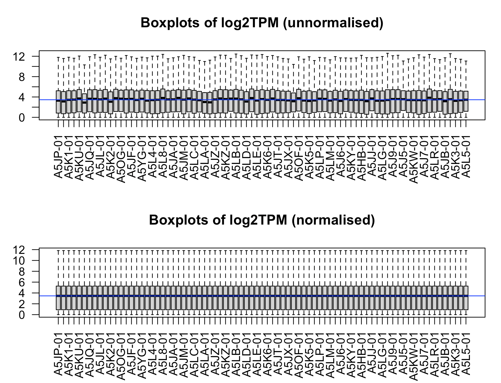
后续也可以对这样的TPM矩阵,进行一些过滤,一些归一化,可视化比如:
代码如下所示:
# Removing genes that are not expressed
table(rowSums(mat_tpm==0)== dim(mat_tpm)[2])
# Which values in mat_tpm are greater than 0
keep.exprs <- mat_tpm > 0
# This produces a logical matrix with TRUEs and FALSEs
head(keep.exprs)
# Summary of how many TRUEs there are in each row
table(rowSums(keep.exprs))
# we would like to keep genes that have at least 2 TRUES in each row of thresh
# keep <- rowSums(keep.exprs) >= round(dim(mat_tpm)[2]*0.1)
# keep <- rowSums(keep.exprs) >= 0
keep <- rowSums(keep.exprs) > 0
summary(keep)
# Subset the rows of countdata to keep the more highly expressed genes
mat_tpm.filtered <- mat_tpm[keep,]
rm(keep.exprs)
rm(eff_length)
mat_tpm.filtered[1:4,1:4]

#--------------------TPM boxplot---------------#
################################################
############## normalize.quantiles #############
################################################
par(mfrow=c(2,1));
# unnormalised
boxplot(log2(mat_tpm.filtered+1),xlab="",ylab="Log2 transcript per million unnormalised",las=2,outline = F)
# Let's add a blue horizontal line that corresponds to the median log2TPM
abline(h=median(log2(mat_tpm.filtered+1)),col="blue")
title("Boxplots of log2TPM (unnormalised)")
# normalised
library(preprocessCore)
mat_tpm.norm<- normalize.quantiles(log2(mat_tpm.filtered+1));
colnames(mat_tpm.norm)<- colnames(mat_tpm.filtered);
rownames(mat_tpm.norm)<- rownames(mat_tpm.filtered);
boxplot(mat_tpm.norm,xlab="",ylab="Log2 transcript per million normalised",las=2,outline = F)
abline(h=median(mat_tpm.norm),col="blue")
title("Boxplots of log2TPM (normalised)")

write.table(mat_tpm.filtered,file = "mat_tpm_filtered.txt",quote = FALSE,sep = "\t")
write.table(mat_tpm.norm,file = "mat_tpm_norm.txt",quote = FALSE,sep = "\t")
save(mat_tpm.norm,file = "mat_tpm_norm.Rdata")