CNS图表复现第二波开启

前面的CNS图表复现专辑，我们写了20个笔记并且分享给大家了，见目录：

当时为了配合文献自己的GitHub代码和数据，我全程没有加入自己的单细胞数据处理标准流程，这样才能把一个简单的降维聚类分群写成20个笔记。

实际上，如果使用我们一直分享的标准代码，就一次性完成全部的步骤，代码如下所示：

step1导入数据

单细胞表达量矩阵总共有6种不同方式导入到R里面构建对象，本文是csv文件，所以代码如下：

###### step1:导入数据 ###### 
rm(list=ls())
options(stringsAsFactors = F)
library(Seurat)
library(ggplot2)
library(clustree)
library(cowplot)
library(dplyr)
# remotes::install_github('chris-mcginnis-ucsf/DoubletFinder') 
# remotes::install_github('immunogenomics/harmony')

# 单细胞项目：来自于30个病人的49个组织样品，跨越3个治疗阶段

# Single-cell RNA sequencing (scRNA-seq) of
# metastatic lung cancer was performed using 49 clinical biopsies obtained from 30 patients before and during
# targeted therapy.

# before initiating systemic targeted therapy (TKI naive [TN]), 
# at the residual disease (RD) state,
# acquired drug resistance (progression [PD]).

library(data.table)
f="Data_input/csv_files/S01_datafinal.csv"
a=fread(f,data.table = F)
a[1:4,1:4]
tail(a[,1:4])
raw.data=a[,-1]
dim(raw.data) # 
rownames(raw.data)=a[,1]
# Load metadata 
f="Data_input/csv_files/S01_metacells.csv"
metadata <- read.csv( f, row.names=1, header=T)
head(metadata) 
row.names(metadata) <- metadata$cell_id 
sce1=CreateSeuratObject(counts = raw.data, 
 meta.data = metadata)
sce1
sce.all=sce1
as.data.frame(sce.all@assays$RNA@counts[1:10, 1:5])
head(sce.all@meta.data, 10)
sce.all@meta.data$orig.ident=sce.all@meta.data$sample_name
table(sce.all@meta.data$orig.ident) 
head(sce.all@meta.data)
#saveRDS(sce.all,file="sce.all_raw.rds")

全程只需要注意 Data_input/csv_files/S01_datafinal.csv 这个文件名路径即可，它在文章的GitHub里面有描述，在作者自己的Dropbox里面。

文章发表在CELL杂志的：Therapy-Induced Evolution of Human Lung Cancer Revealed by Single-Cell RNA Sequencing 。全套代码在：https://github.com/czbiohub/scell_lung_adenocarcinoma

step2: 质量控制

主要是看看核糖体基因比例，线粒体基因以及红细胞基因，然后看看表达量比较高的top50基因，以及细胞周期。


#rm(list=ls())
###### step2:QC质控 ######
dir.create("./1-QC")
setwd("./1-QC")
# sce.all=readRDS("../sce.all_raw.rds")
#计算线粒体基因比例
# 人和鼠的基因名字稍微不一样 
mito_genes=rownames(sce.all)[grep("^ERCC-", rownames(sce.all))] 
mito_genes #13个线粒体基因
sce.all=PercentageFeatureSet(sce.all, "^ERCC-", col.name = "percent_mito")
fivenum(sce.all@meta.data$percent_mito)
#计算核糖体基因比例
ribo_genes=rownames(sce.all)[grep("^Rp[sl]", rownames(sce.all),ignore.case = T)]
ribo_genes
sce.all=PercentageFeatureSet(sce.all, "^RP[SL]", col.name = "percent_ribo")
fivenum(sce.all@meta.data$percent_ribo)
#计算红血细胞基因比例
rownames(sce.all)[grep("^Hb[^(p)]", rownames(sce.all),ignore.case = T)]
sce.all=PercentageFeatureSet(sce.all, "^HB[^(P)]", col.name = "percent_hb")
fivenum(sce.all@meta.data$percent_hb)
#可视化细胞的上述比例情况
feats <- c("nFeature_RNA", "nCount_RNA", "percent_mito", "percent_ribo", "percent_hb")
feats <- c("nFeature_RNA", "nCount_RNA")
p1=VlnPlot(sce.all, group.by = "orig.ident", features = feats, pt.size = 0.01, ncol = 2) + 
 NoLegend()
p1
library(ggplot2) 
ggsave(filename="Vlnplot1.png",plot=p1)
feats <- c("percent_mito", "percent_ribo", "percent_hb")
p2=VlnPlot(sce.all, group.by = "orig.ident", features = feats, pt.size = 0.01, ncol = 3, same.y.lims=T) + 
 scale_y_continuous(breaks=seq(0, 100, 5)) +
 NoLegend()
p2 
ggsave(filename="Vlnplot2.pdf",plot=p2)

p3=FeatureScatter(sce.all, "nCount_RNA", "nFeature_RNA", group.by = "orig.ident", pt.size = 0.5)
ggsave(filename="Scatterplot.pdf",plot=p3)
#根据上述指标，过滤低质量细胞/基因
#过滤指标1:最少表达基因数的细胞&最少表达细胞数的基因
selected_c <- WhichCells(sce.all, expression = nFeature_RNA > 300)
selected_f <- rownames(sce.all)[Matrix::rowSums(sce.all@assays$RNA@counts > 0 ) > 3]

sce.all.filt <- subset(sce.all, features = selected_f, cells = selected_c)
dim(sce.all) 
dim(sce.all.filt)

# 可以看到，主要是过滤了基因，其次才是细胞

# par(mar = c(4, 8, 2, 1))
C=sce.all.filt@assays$RNA@counts
dim(C)
C=Matrix::t(Matrix::t(C)/Matrix::colSums(C)) * 100
# 这里的C 这个矩阵，有一点大，可以考虑随抽样
C=C[,sample(1:ncol(C),1000)]
most_expressed <- order(apply(C, 1, median), decreasing = T)[50:1]
pdf("TOP50_most_expressed_gene.pdf",width=14)
boxplot(as.matrix(Matrix::t(C[most_expressed, ])),
 cex = 0.1, las = 1, 
 xlab = "% total count per cell", 
 col = (scales::hue_pal())(50)[50:1], 
 horizontal = TRUE)
dev.off()
rm(C)

#过滤指标2:线粒体/核糖体基因比例(根据上面的violin图)
selected_mito <- WhichCells(sce.all.filt, expression = percent_mito < 20)
selected_ribo <- WhichCells(sce.all.filt, expression = percent_ribo > 3)
selected_hb <- WhichCells(sce.all.filt, expression = percent_hb < 0.1)
length(selected_hb)
length(selected_ribo)
length(selected_mito)

sce.all.filt <- subset(sce.all.filt, cells = selected_mito)
#sce.all.filt <- subset(sce.all.filt, cells = selected_ribo)
sce.all.filt <- subset(sce.all.filt, cells = selected_hb)
dim(sce.all.filt)

table(sce.all.filt$orig.ident) 
#可视化过滤后的情况
feats <- c("nFeature_RNA", "nCount_RNA")
p1_filtered=VlnPlot(sce.all.filt, group.by = "orig.ident", features = feats, pt.size = 0.1, ncol = 2) + 
 NoLegend()
ggsave(filename="Vlnplot1_filtered.pdf",plot=p1_filtered)

feats <- c("percent_mito", "percent_ribo", "percent_hb")
p2_filtered=VlnPlot(sce.all.filt, group.by = "orig.ident", features = feats, pt.size = 0.1, ncol = 3) + 
 NoLegend()
ggsave(filename="Vlnplot2_filtered.pdf",plot=p2_filtered)

#过滤指标3:过滤特定基因
# Filter MALAT1 管家基因
sce.all.filt <- sce.all.filt[!grepl("MALAT1", rownames(sce.all.filt),ignore.case = T), ]
# Filter Mitocondrial 线粒体基因
sce.all.filt <- sce.all.filt[!grepl("^ERCC-", rownames(sce.all.filt),ignore.case = T), ]
# 当然，还可以过滤更多

dim(sce.all.filt)

#细胞周期评分
sce.all.filt = NormalizeData(sce.all.filt)
s.genes=Seurat::cc.genes.updated.2019$s.genes
g2m.genes=Seurat::cc.genes.updated.2019$g2m.genes
sce.all.filt=CellCycleScoring(object = sce.all.filt, 
 s.features = s.genes, 
 g2m.features = g2m.genes, 
 set.ident = TRUE)
p4=VlnPlot(sce.all.filt, features = c("S.Score", "G2M.Score"), group.by = "orig.ident", 
 ncol = 2, pt.size = 0.1)
ggsave(filename="Vlnplot4_cycle.pdf",plot=p4)

sce.all.filt@meta.data %>% ggplot(aes(S.Score,G2M.Score))+geom_point(aes(color=Phase))+
 theme_minimal()
ggsave(filename="cycle_details.pdf" )
# S.Score较高的为S期，G2M.Score较高的为G2M期，都比较低的为G1期

质量控制绝大部分情况下都是跑一下而已，很少需要仔细看，因为单细胞转录组目前是比较稳定的，如果数据有问题，给你服务的公司也会提醒你。

step3：多个分辨率降维聚类分群

 # 前面已经跑了 NormalizeData 步骤哦！
sce.all.filt = FindVariableFeatures(sce.all.filt)
sce.all.filt = ScaleData(sce.all.filt, 
 vars.to.regress = c("nFeature_RNA", "percent_mito"))
sce.all.filt = RunPCA(sce.all.filt, npcs = 20)
sce.all.filt = RunTSNE(sce.all.filt, npcs = 20)
sce.all.filt = RunUMAP(sce.all.filt, dims = 1:10)
# define the expected number of doublet cells cells. 
dim(sce.all.filt) 
dim(sce.all)

setwd('../')
dir.create("2-int")
getwd()
setwd("2-int")
# sce.all=readRDS("../1-QC/sce.all_qc.rds")
sce.all=sce.all.filt
sce.all
#拆分为 个seurat子对象
sce.all.list <- SplitObject(sce.all, split.by = "orig.ident")
sce.all.list
length(sce.all.list)

# 对 smart-seq2 技术的单细胞， CCA整合并没有必要 
sce.all
sce.all@active.assay
sce.all=FindNeighbors(sce.all, dims = 1:10, k.param = 60, prune.SNN = 1/15)
#设置不同的分辨率，观察分群效果(选择哪一个？)
for (res in c(0.01, 0.05, 0.1, 0.2, 0.3, 0.5,0.8,1)) {
 sce.all=FindClusters(sce.all, #graph.name = "CCA_snn", 
 resolution = res, algorithm = 1)
}
colnames(sce.all@meta.data)
apply(sce.all@meta.data[,grep("RNA_snn",colnames(sce.all@meta.data))],2,table)

p1_dim=plot_grid(ncol = 3, DimPlot(sce.all, reduction = "umap", group.by = "RNA_snn_res.0.01") + 
 ggtitle("louvain_0.01"), DimPlot(sce.all, reduction = "umap", group.by = "RNA_snn_res.0.1") + 
 ggtitle("louvain_0.1"), DimPlot(sce.all, reduction = "umap", group.by = "RNA_snn_res.0.2") + 
 ggtitle("louvain_0.2"))
ggsave(plot=p1_dim, filename="Dimplot_diff_resolution_low.pdf",width = 14)

p1_dim=plot_grid(ncol = 3, DimPlot(sce.all, reduction = "umap", group.by = "RNA_snn_res.0.8") + 
 ggtitle("louvain_0.8"), DimPlot(sce.all, reduction = "umap", group.by = "RNA_snn_res.1") + 
 ggtitle("louvain_1"), DimPlot(sce.all, reduction = "umap", group.by = "RNA_snn_res.0.3") + 
 ggtitle("louvain_0.3"))
ggsave(plot=p1_dim, filename="Dimplot_diff_resolution_high.pdf",width = 18)

p2_tree=clustree(sce.all@meta.data, prefix = "RNA_snn_res.")
ggsave(plot=p2_tree, filename="Tree_diff_resolution.pdf")

#接下来分析，按照分辨率为0.8进行 
sel.clust = "RNA_snn_res.0.8"
sce.all <- SetIdent(sce.all, value = sel.clust)
table(sce.all@active.ident) 
saveRDS(sce.all, "sce.all_int.rds")

step4:检查常见分群情况

代码有点长，因为我内置了多个基因列表，在初始的分辨率为0.8的分群结果下，批量检查它们的表达量情况！


dir.create("../3-cell")
setwd("../3-cell")

rm(list=ls())
options(stringsAsFactors = F)
library(Seurat)
library(ggplot2)
library(clustree)
library(cowplot)
library(dplyr)
getwd()
setwd('3-cell/')
sce.all=readRDS( "../2-int/sce.all_int.rds")
sce.all

DimPlot(sce.all, reduction = "umap", group.by = "seurat_clusters",label = T) 
DimPlot(sce.all, reduction = "umap", group.by = "RNA_snn_res.0.8",label = T) 
ggsave('umap_by_RNA_snn_res.0.8.pdf')

# Tumor cells were identified using MLANA, MITF, and DCT.
# Tumor cells were further divided into subgroups 
# by expression of PRAME and GEP genes

library(ggplot2) 
genes_to_check = c('PTPRC', 'CD3D', 'CD3E', # T cells
 'KLRD1', # natural killer (NK) cells
 'FCGR3B', #neutrophils
 'MS4A1' ,'IGHG4', # b cells 
 'RPE65','RCVRN',
 'CD68', 'CD163', 'CD14', 'MKI67' ,'TOP2A',
 'MLANA', 'MITF', 'DCT','PRAME' , 'GEP' )
library(stringr) 
p_paper_markers <- DotPlot(sce.all, features = genes_to_check,
 assay='RNA' ) + coord_flip()

p_paper_markers
ggsave(plot=p_paper_markers,
 filename="check_paper_marker_by_seurat_cluster.pdf",width = 12)

# T Cells (CD3D, CD3E, CD8A), 
# B cells (CD19, CD79A, MS4A1 [CD20]), 
# Plasma cells (IGHG1, MZB1, SDC1, CD79A), 
# Monocytes and macrophages (CD68, CD163, CD14),
# NK Cells (FGFBP2, FCG3RA, CX3CR1), 
# Photoreceptor cells (RCVRN), 
# Fibroblasts (FGF7, MME), 
# Endothelial cells (PECAM1, VWF). 
# epi or tumor (EPCAM, KRT19, PROM1, ALDH1A1, CD24).
# immune (CD45+,PTPRC), epithelial/cancer (EpCAM+,EPCAM), 
# stromal (CD10+,MME,fibo or CD31+,PECAM1,endo)

library(ggplot2) 
genes_to_check = c('PTPRC', 'CD3D', 'CD3E', 'CD4','CD8A','CD19', 'CD79A', 'MS4A1' ,
 'IGHG1', 'MZB1', 'SDC1',
 'CD68', 'CD163', 'CD14', 
 'TPSAB1' , 'TPSB2', # mast cells,
 'RCVRN','FPR1' , 'ITGAM' ,
 'FGF7','MME', 'ACTA2',
 'PECAM1', 'VWF', 
 'EPCAM' , 'KRT19', 'PROM1', 'ALDH1A1' )
library(stringr) 
p_all_markers <- DotPlot(sce.all, features = genes_to_check,
 assay='RNA' ) + coord_flip()

p_all_markers
ggsave(plot=p_all_markers, filename="check_all_marker_by_seurat_cluster.pdf")

genes_to_check = c('PTPRC', 'CD3D', 'CD3E', 'CD4','CD8A',
 'CCR7', 'SELL' , 'TCF7','CXCR6' , 'ITGA1',
 'FOXP3', 'IL2RA', 'CTLA4','GZMB', 'GZMK','CCL5',
 'IFNG', 'CCL4', 'CCL3' ,
 'PRF1' , 'NKG7') 
library(stringr) 
p <- DotPlot(sce.all, features = genes_to_check,
 assay='RNA' ) + coord_flip()

p
ggsave(plot=p, filename="check_Tcells_marker_by_seurat_cluster.pdf")

# mast cells, TPSAB1 and TPSB2 
# B cell, CD79A and MS4A1 (CD20) 
# naive B cells, such as MS4A1 (CD20), CD19, CD22, TCL1A, and CD83, 
# plasma B cells, such as CD38, TNFRSF17 (BCMA), and IGHG1/IGHG4
genes_to_check = c('CD3D','MS4A1','CD79A',
 'CD19', 'CD22', 'TCL1A', 'CD83', # naive B cells
 'CD38','TNFRSF17','IGHG1','IGHG4', # plasma B cells,
 'TPSAB1' , 'TPSB2', # mast cells,
 'PTPRC' ) 
p <- DotPlot(sce.all, features = genes_to_check,
 assay='RNA' ) + coord_flip()

p
ggsave(plot=p, filename="check_Bcells_marker_by_seurat_cluster.pdf")

genes_to_check = c('CD68', 'CD163', 'CD14', 'CD86', 'LAMP3', ## DC 
 'CD68', 'CD163','MRC1','MSR1','ITGAE','ITGAM','ITGAX','SIGLEC7', 
 'MAF','APOE','FOLR2','RELB','BST2','BATF3')
p <- DotPlot(sce.all, features = unique(genes_to_check),
 assay='RNA' ) + coord_flip()

p
ggsave(plot=p, filename="check_Myeloid_marker_by_seurat_cluster.pdf")

# epi or tumor (EPCAM, KRT19, PROM1, ALDH1A1, CD24).
# - alveolar type I cell (AT1; AGER+)
# - alveolar type II cell (AT2; SFTPA1)
# - secretory club cell (Club; SCGB1A1+)
# - basal airway epithelial cells (Basal; KRT17+)
# - ciliated airway epithelial cells (Ciliated; TPPP3+)

genes_to_check = c( 'EPCAM' , 'KRT19', 'PROM1', 'ALDH1A1' ,
 'AGER','SFTPA1','SCGB1A1','KRT17','TPPP3',
 'KRT4','KRT14','KRT8','KRT18',
 'CD3D','PTPRC' ) 
p <- DotPlot(sce.all, features = unique(genes_to_check),
 assay='RNA' ) + coord_flip()

p
ggsave(plot=p, filename="check_epi_marker_by_seurat_cluster.pdf")

genes_to_check = c('TEK',"PTPRC","EPCAM","PDPN","PECAM1",'PDGFRB',
 'CSPG4','GJB2', 'RGS5','ITGA7',
 'ACTA2','RBP1','CD36', 'ADGRE5','COL11A1','FGF7', 'MME')
p <- DotPlot(sce.all, features = unique(genes_to_check),
 assay='RNA' ) + coord_flip()

p
ggsave(plot=p, filename="check_stromal_marker_by_seurat_cluster.pdf")

p_all_markers
p_umap=DimPlot(sce.all, reduction = "umap",
 group.by = "RNA_snn_res.0.8",label = T) 
library(patchwork)
p_all_markers+p_umap
ggsave('markers_umap.pdf',width = 15)
DimPlot(sce.all, reduction = "umap",split.by = 'orig.ident',
 group.by = "RNA_snn_res.0.8",label = T) 
ggsave('orig.ident_umap.pdf')

如下所示：

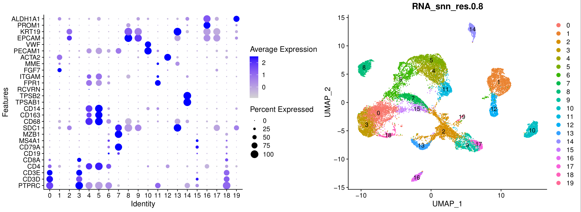
如果有生物学背景，很容易根据这些基因名字，对原始的单细胞亚群进行合并和生物学命名。

也可以顺便看看原始分群各自的高表达量基因哦，代码如下所示：

sce.all 
sce=sce.all
table(Idents(sce)) 
sce.markers <- FindAllMarkers(object = sce, only.pos = TRUE, min.pct = 0.25, 
 thresh.use = 0.25)
DT::datatable(sce.markers)

pro='RNA_snn_res.0.8'
write.csv(sce.markers,file=paste0(pro,'_sce.markers.csv'))
library(dplyr) 
top10 <- sce.markers %>% group_by(cluster) %>% top_n(10, avg_log2FC)
DoHeatmap(sce,top10$gene,size=3)
ggsave(filename=paste0(pro,'_sce.markers_heatmap.pdf'))

library(dplyr) 
top3 <- sce.markers %>% group_by(cluster) %>% top_n(3, avg_log2FC)
DoHeatmap(sce,top3$gene,size=3)
ggsave(paste0(pro,'DoHeatmap_check_top3_markers_by_clusters.pdf'))
p <- DotPlot(sce, features = unique(top3$gene),
 assay='RNA' ) + coord_flip()

p
ggsave(paste0(pro,'DotPlot_check_top3_markers_by_clusters.pdf'))
save(sce.markers,file = 'sce.markers.Rdata')

各个亚群自己的高表达量基因可以辅助我们进行单细胞亚群的生物学命名。

step5: 人工命名生物学单细胞亚群


celltype=data.frame(ClusterID=0:19,
 celltype=0:19) 
celltype[celltype$ClusterID %in% c( 2,9,13,16,17,19,8),2]='epi' 
celltype[celltype$ClusterID %in% c( 7,15 ),2]='B' 
celltype[celltype$ClusterID %in% c( 14),2]='Mast' 
celltype[celltype$ClusterID %in% c( 0,3,18 ),2]='T' 
celltype[celltype$ClusterID %in% c( 4,5,6,11 ),2]='myeloid' 
celltype[celltype$ClusterID %in% c( 10),2]='endo' 
celltype[celltype$ClusterID %in% c( 1,12),2]='fibo'

head(celltype)
celltype 
table(celltype$celltype)
sce.all@meta.data$celltype = "NA"
for(i in 1:nrow(celltype)){
 sce.all@meta.data[which(sce.all@meta.data$RNA_snn_res.0.8 == celltype$ClusterID[i]),'celltype'] <- celltype$celltype[i]}
table(sce.all@meta.data$celltype)

genes_to_check = c('PTPRC', 'CD3D', 'CD3E', 'CD4','CD8A','CD19', 'CD79A', 'MS4A1' ,
 'IGHG1', 'MZB1', 'SDC1',
 'CD68', 'CD163', 'CD14', 
 'TPSAB1' , 'TPSB2', # mast cells,
 'RCVRN','FPR1' , 'ITGAM' ,
 'FGF7','MME', 'ACTA2',
 'PECAM1', 'VWF', 
 'EPCAM' , 'KRT19', 'PROM1', 'ALDH1A1' )
p <- DotPlot(sce.all, features = genes_to_check,
 assay='RNA' ,group.by = 'celltype' ) + coord_flip()

p
ggsave(plot=p, filename="check_marker_by_celltype.pdf")
table(sce.all@meta.data$celltype,sce.all@meta.data$RNA_snn_res.0.8)

DimPlot(sce.all, reduction = "umap", group.by = "celltype",label = T) 
ggsave('umap_by_celltype.pdf')

library(patchwork)

p_all_markers=DotPlot(sce.all, features = genes_to_check,
 assay='RNA' ,group.by = 'celltype' ) + coord_flip()
p_umap=DimPlot(sce.all, reduction = "umap", group.by = "celltype",label = T) 
p_all_markers+p_umap
ggsave('markers_umap_by_celltype.pdf',width = 13)
phe=sce.all@meta.data
save(phe,file = 'phe_by_markers.Rdata')

如下所示：

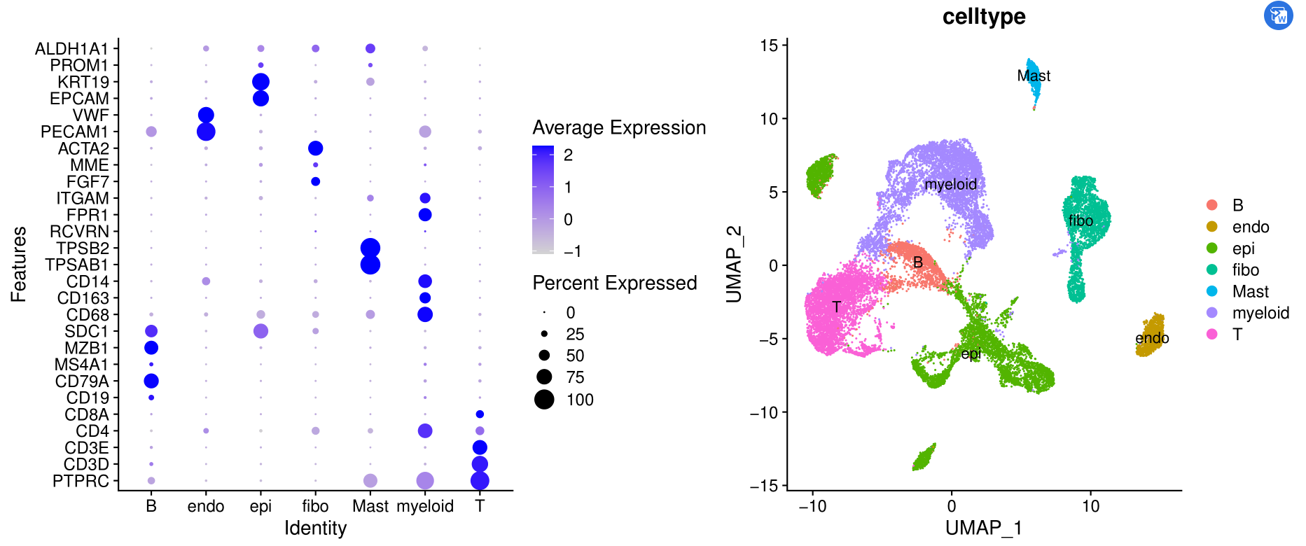
这个是初步的降维聚类分群啦，而且给出来了生物学名字。

它虽然不完美，但是拿到了单细胞表达量矩阵，先跑一下这个流程，还是很大程度能帮助我们理解自己的单细胞数据哦！

可以看到不同亚群的高表达量基因以及各自的比例情况。

生信菜鸟团

欢迎去论坛biotrainee.com留言参与讨论，或者关注同名微信公众号biotrainee