又一次被迫讨论这个让人又爱又恨的批次效应了,主要是因为上一个教程 不同癌症的差异难道大于其与正常对照差异吗:大家的留言:
我们这一次的主题就是 探索 不同癌症的正常对照,有没有可能通过去除批次效应或者其它处理来让他们的距离更近,这次我们的结论是:其实有些批次效应是不可能被矫正的!
首先尝试使用harmony 抹去癌症差异
代码如下所示:
# 其中 sce 对象来源于前面的系列教程哦: https://mp.weixin.qq.com/s/p2oYAgG-LO9yLGx1r3i9zQ

table( sce$group)
library(harmony)
seuratObj <- RunHarmony(sce, "group")
names(seuratObj@reductions)
seuratObj <- RunUMAP(seuratObj, dims = 1:15,
 reduction = "harmony")
DimPlot(seuratObj,reduction = "umap",label=T ) +NoLegend()
library(cowplot)
p1.compare=plot_grid(ncol = 3,
 DimPlot(sce, reduction = "pca", group.by = "group")+NoAxes() +NoLegend()+ggtitle("PCA"),
 DimPlot(sce, reduction = "tsne", group.by = "group")+NoAxes() +NoLegend()+ggtitle("tSNE"),
 DimPlot(sce, reduction = "umap", group.by = "group")+NoAxes() +NoLegend()+ggtitle("UMAP"),
 DimPlot(seuratObj, reduction = "pca", group.by = "group")+NoAxes() +NoLegend()+ggtitle("PCA"),
 DimPlot(seuratObj, reduction = "tsne", group.by = "group")+NoAxes() +NoLegend()+ggtitle("tSNE"),
 DimPlot(seuratObj, reduction = "umap", group.by = "group")+NoAxes() +NoLegend()+ggtitle("UMAP")
)
p1.compare
ggsave(plot=p1.compare,filename="before_and_after_inter_cancerType.pdf")
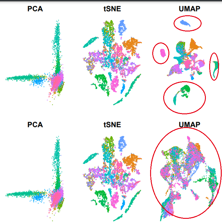
可以很明显的看到harmony的效果:
- 上面的是使用harmony 抹去癌症差异之前,可以看到绝大部分癌症都是独立成群
- 下面的是抹去癌症差异之后,可以看到不同癌症混合在了一起!
仍然需要降维聚类分群
基于harmony 抹去癌症差异后 的表达量矩阵,仍然是需要降维聚类分群哦!
代码如下所示:
sce=seuratObj
sce <- FindNeighbors(sce, reduction = "harmony",dims = 1:15)
sce <- FindClusters(sce, resolution = 0.5)
table(sce@meta.data$seurat_clusters)
DimPlot(sce,reduction = "umap",label=T)
ggsave(filename = 'harmony_umap_recluster_by_0.5.pdf')

p1=DimPlot(sce,reduction = "umap",label=T,
 group.by = 'group')
p1
ggsave(filename = 'harmony_umap_sce_recluster_by_cancerType.pdf')

cl=c('#7fc97f','#beaed4','#fdc086','#ffff99','#386cb0','#f0027f','#bf5b17')
p2=DimPlot(sce,reduction = "umap",label=T,
 cols = cl,
 group.by = 'gp')
p2
ggsave(filename = 'harmony_umap_sce_recluster_by_position.pdf')
library(patchwork)
p1+p2

library(gplots)
balloonplot(table(sce$seurat_clusters,
 sce$gp))

balloonplot(table(sce$seurat_clusters,
 sce$group))
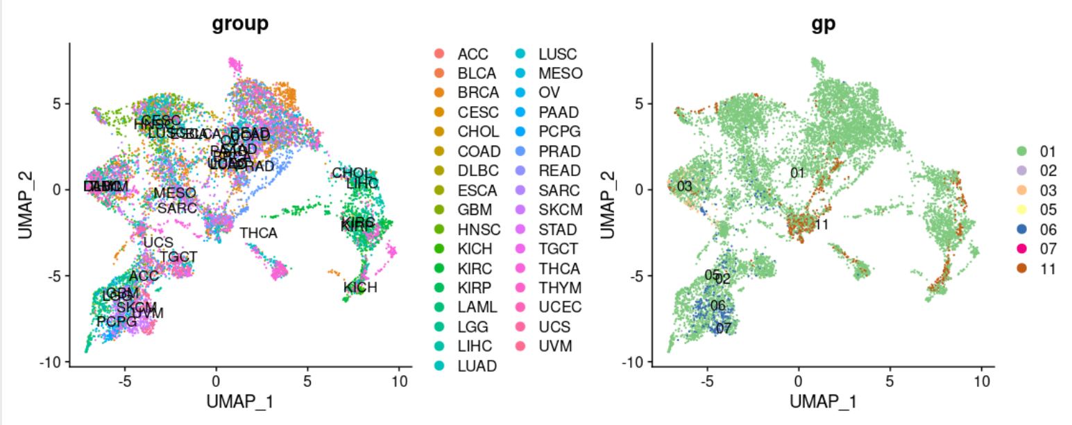
可以看到抹去癌症差异并不会导致正常组织独立成为一个细胞亚群:
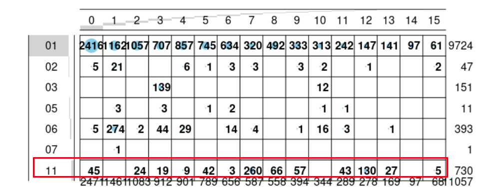
各个癌症确实是混合到了一起:
如果看各个细胞亚群的癌症样品分布,足够强的生物学背景可以帮我们解释下面的图:
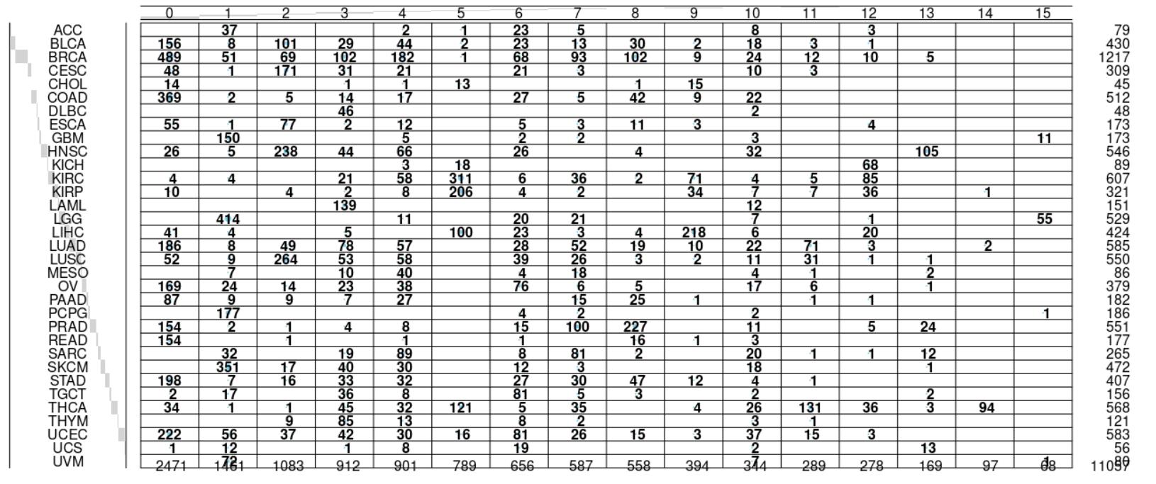
但是目前的我确实看不出一个所以然!
再次寻找各个亚群的特征基因
代码如下:
# 接下来对seurat默认的分群进行差异分析

pro='harmony_seurat-0.5'
table(Idents(sce))
sce.markers <- FindAllMarkers(object = sce, only.pos = TRUE, min.pct = 0.25,
 thresh.use = 0.25)
DT::datatable(sce.markers)
write.csv(sce.markers,file=paste0(pro,'_sce.markers.csv'))
library(dplyr)
top10 <- sce.markers %>% group_by(cluster) %>% top_n(10, avg_log2FC)
DoHeatmap(sce,top10$gene,size=3)
ggsave(filename=paste0(pro,'_sce.markers_heatmap.pdf'),width = 18,height = 21)
p <- DotPlot(sce, features = unique(top10$gene),
 assay='RNA' ) + coord_flip()

p
ggsave(paste0(pro,'-DotPlot_check_top10_markers_by_clusters.pdf'),width = 18,height = 21)

library(dplyr)
top3 <- sce.markers %>% group_by(cluster) %>% top_n(3, avg_log2FC)
DoHeatmap(sce,top3$gene,size=3)
ggsave(paste0(pro,'-DoHeatmap_check_top3_markers_by_clusters.pdf'),width = 18,height = 11)
p <- DotPlot(sce, features = unique(top3$gene),
 assay='RNA' ) + coord_flip()

p
ggsave(paste0(pro,'-DotPlot_check_top3_markers_by_clusters.pdf'),width = 18,height = 11)

save(sce.markers,file=paste0(pro,file = '-sce.markers.Rdata'))
其中各个细胞亚群里面的top3基因的热图如下所示:
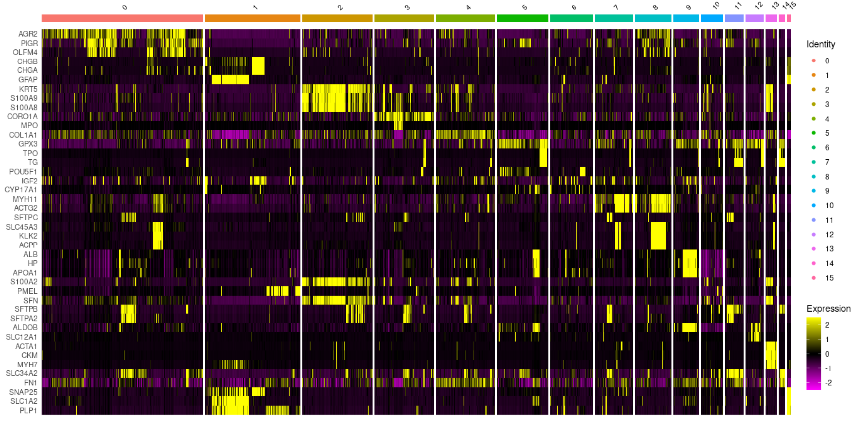
因为确实不是真正的单细胞,里面的基因并不是我们耳熟能详的单细胞标记基因,而且分组太多,每个组都有成百上千个基因,肉眼不可能一一检查, 这个时候可以做各亚群特征基因的kegg数据库富集分析。
各亚群特征基因的kegg数据库富集分析
代码如下所示:
table(sce.markers$cluster)
library(org.Hs.eg.db)
library(clusterProfiler)
ids=bitr(sce.markers$gene,'SYMBOL','ENTREZID','org.Hs.eg.db')
sce.markers=merge(sce.markers,ids,by.x='gene',by.y='SYMBOL')
gcSample=split(sce.markers$ENTREZID, sce.markers$cluster)
gcSample # entrez id , compareCluster
xx <- compareCluster(gcSample, fun="enrichKEGG",
 organism="hsa", pvalueCutoff=0.05)
p=dotplot(xx)
p+ theme(axis.text.x = element_text(angle = 45,
 vjust = 0.5, hjust=0.5))
p
可以看到,还是蛮有意思的:
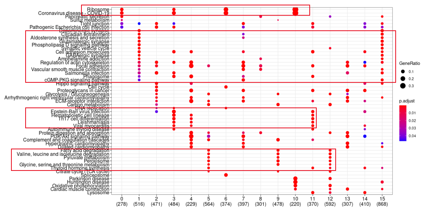
其中,第 0,3,6,10是核糖体高表达的癌症样品,它们也跨越了多个细胞亚群!
这个时候可以延伸出很多课题:
- 核糖体高表达的癌症是否预后更差?
- S100A8,S100A9这样的monocytes标记基因为什么和KRT5一样特异性出现在第2群?
更多课题都可以看这个比较里面的图片啦,就需要你们有有一双善于发现美的眼睛!
欢迎加入我们的交流群, 详见:https://mp.weixin.qq.com/s/rwlZadSu-xnuoPK1nGnPIg