今天介绍的文章是2021年1月发表在cancer research杂志 : 《Single-Cell Transcriptomic Heterogeneity in Invasive Ductal and Lobular Breast Cancer Cells》,链接是 https://pubmed.ncbi.nlm.nih.gov/33148662/
这个数据的研究目标是:To quantify ITH between cell lines, referred to as ICH (Inter-Cellular Heterogeneity), and investigate differences between IDC and ILC,:
- Invasive lobular breast carcinoma (ILC),
- Invasive ductal cancer subtype (IDC).
数据链接是:https://www.ncbi.nlm.nih.gov/geo/query/acc.cgi?acc=GSE144320
只有一个10X样品样本:
GSM4285803 All_CellLines
作者提供了该样本的三个文件,但并不是我们通常说的10x的3个文件:
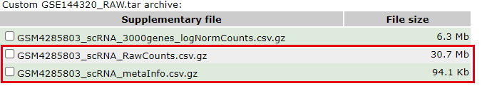
这个单细胞文章仅仅是单个10X样品,但是测8个细胞系。
- MCF7 (n=977)
- T47D WT (n=509)
- T47D KO (n=491)
- MM134 (n=439)
- SUM44 (n=314)
- BCK4 (n=512)
- MCF10A (n=491)
- HEK293T(n=881).
作者使用六个公共数据集来进行建立参考数据集与自己的数据进行相关性分析,进行细胞注释:
1,444 genes were present in all the three data sources (breast cell lines, HEK293T as reference 186 cell lines;
and scRNA-seq (3,000 genes by 4,614 cells) as query cells);
Two external datasets with scRNA-seq data of cell lines were integrated with our data for CNA inference - MCF7 and T47D cells from Hong et al.(29), and three MCF7 strains (WT-3,4,5) from Ben-David et al;
A raw count matrix from Hong et al was directly downloaded from GSE122743 while FASTQ files from Ben-David
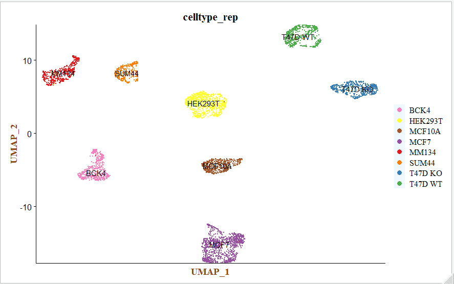
本次要复现的文献图表如下所示:
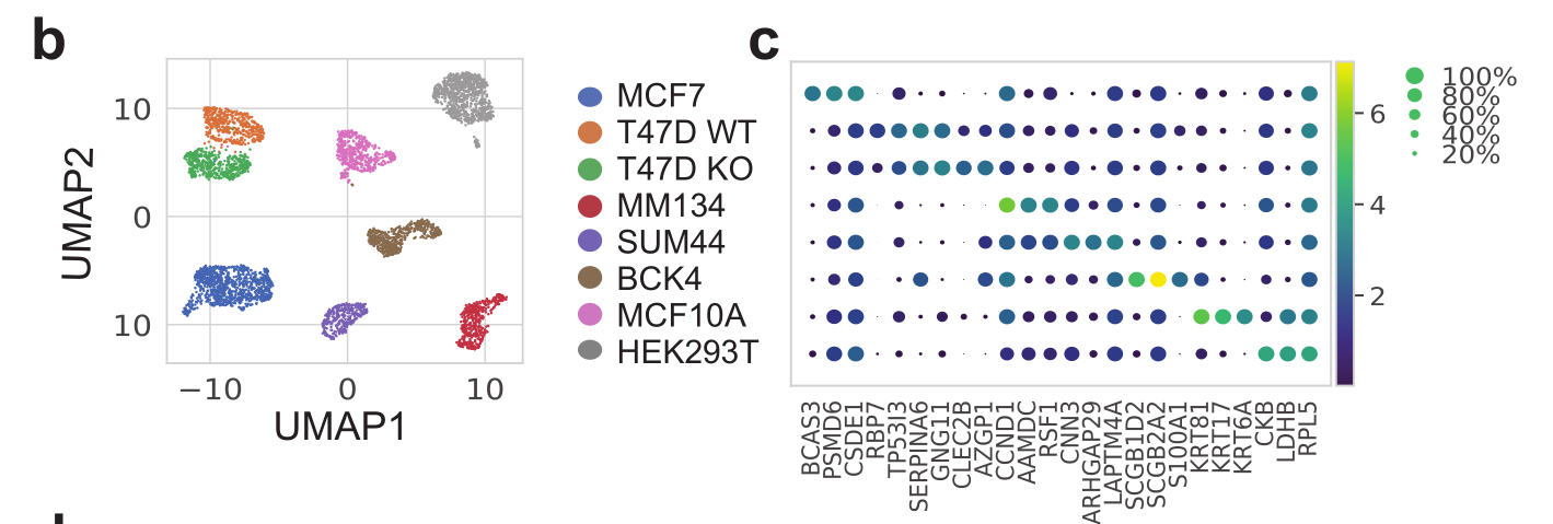
是单细胞转录组数据分析的标准降维聚类分群,并且进行生物学注释后的结果。可以参考前面的例子:人人都能学会的单细胞聚类分群注释 ,我们演示了第一层次的分群。
如果你对单细胞数据分析还没有基础认知,可以看基础10讲:
- 01. 上游分析流程
- 02.课题多少个样品,测序数据量如何
- 03. 过滤不合格细胞和基因(数据质控很重要)
- 04. 过滤线粒体核糖体基因
- 05. 去除细胞效应和基因效应
- 06.单细胞转录组数据的降维聚类分群
- 07.单细胞转录组数据处理之细胞亚群注释
- 08.把拿到的亚群进行更细致的分群
- 09.单细胞转录组数据处理之细胞亚群比例比较
下面我们开始复现:
在运行环境下创建一个GSE144320_RAW文件夹,里面包含下面两个文件:

step1:读取表达矩阵文件,然后构建Seurat对象
构建Seurat对象后保存为 sce.Rds 文件,供后续使用
suppressPackageStartupMessages(library(Seurat))
suppressPackageStartupMessages(library(ggplot2))
suppressPackageStartupMessages(library(clustree))
suppressPackageStartupMessages(library(cowplot))
suppressPackageStartupMessages(library(dplyr))
suppressPackageStartupMessages(library(data.table))

# 构建seurat对象
# 读取rawcounts矩阵
a <- textshape::column_to_rownames(fread("../GSE144320_RAW/GSM4285803_scRNA_RawCounts.csv.gz"),
 loc = 1)
sce <- CreateSeuratObject(counts = as.data.frame(t(a)))
# 计算线粒体基因比例
(mito_genes <- rownames(sce[grep("^MT-", rownames(sce))]))
sce <- PercentageFeatureSet(sce, "^MT-", col.name = "percent_Mito_rep")
sce@meta.data$percent_Mito_rep[1:6]
head(sce@meta.data)
#计算周期评分
sce = NormalizeData(sce)
sce <- CellCycleScoring(sce,
 g2m.features = cc.genes$g2m.genes,
 s.features = cc.genes$s.genes)
# 读取文章meta信息
meta <- fread("../GSE144320_RAW/GSM4285803_scRNA_metaInfo.csv.gz")
meta <- textshape::column_to_rownames(meta, 1)
#将作者提供表型信息添加到seurat对象中
sce <- AddMetaData(sce, metadata = meta)
# 保存数据
saveRDS(sce, file = "sce.Rds")
step2: 降维聚类分群
仍然是面的例子:人人都能学会的单细胞聚类分群注释 ,
##### step2 降维聚类分群#####
#读入数据
sce <- readRDS("sce.Rds")
#数据预处理

sce <- FindVariableFeatures(sce, nfeatures = 3000)
sce
# 默认后续使用 HVGs 进行 特征寻找
sce = ScaleData(sce
 # features = rownames(sce),
 #vars.to.regress = c("nFeature_RNA", "percent_mito")
) #加上vars.to.regress参数后运行so slow!!!
# 降维处理
sce <- RunPCA(sce, npcs = 30)
sce <- RunTSNE(sce, dims = 1:30)
sce <- RunUMAP(sce, dims = 1:30)

# 聚类分析
sce <- FindNeighbors(sce, dims = 1:30)
for (res in c(0.01, 0.05, 0.1, 0.2, 0.3, 0.5,0.8,1)) {
 sce <- FindClusters(sce, graph.name = "RNA_snn", resolution = res, algorithm = 1)
}
ls <- apply(sce@meta.data[,grep("RNA_snn_res",colnames(sce@meta.data))],2,table)
#聚类树可视化
colors <- c('#e41a1c','#377eb8','#4daf4a','#984ea3','#ff7f00','#ffff33','#a65628','#f781bf')
names(colors) <- unique(colnames(sce@meta.data)[grep("RNA_snn_res", colnames(sce@meta.data))])

p2_tree <- clustree(sce@meta.data, prefix = "RNA_snn_res.")
p2_tree
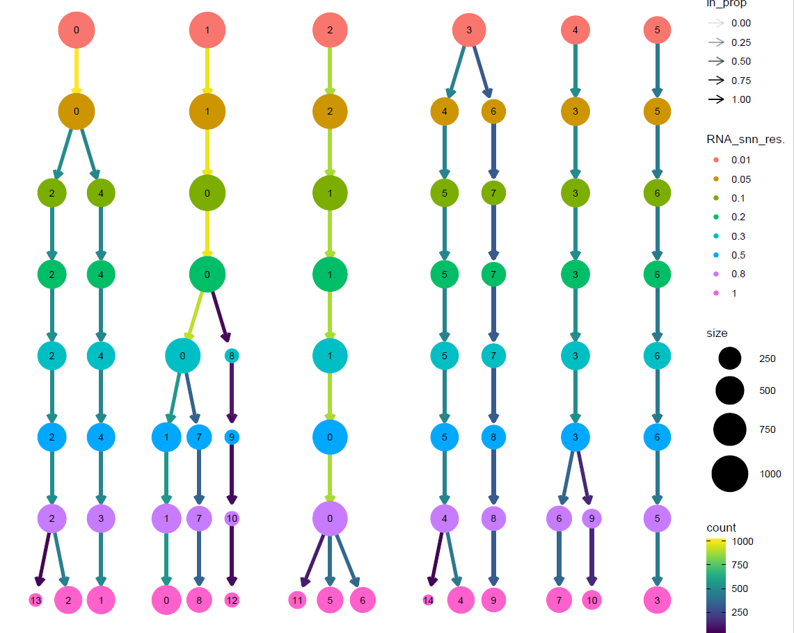
文献里面提到了是8个不同细胞系,所以我们这里使用resolution = 0.2 进行后续分析即可。
# 取resolution = 0.2 进行后续分析
colors <- c('#e41a1c','#377eb8','#4daf4a','#984ea3','#ff7f00','#ffff33','#a65628','#f781bf')
p <- DimPlot(sce, reduction = "umap", group.by = "RNA_snn_res.0.2", label = T, cols = colors)+
 scale_y_continuous(expand = c(0, 0)) +
 scale_x_discrete(position = "bottom") +
 scale_fill_manual( breaks = rev(names(colors)),values = colors) +
 theme(
 plot.title = element_text(family = "serif", hjust = 0.5, vjust = 0, colour = "black"),
 # 坐标轴标题
 axis.title.x = element_text(family = "serif",face = "bold",colour = "chocolate4", hjust = 0.5, vjust = 0),
 axis.title.y = element_text(family = "serif",face = "bold",colour = "chocolate4", hjust = 0.5, vjust = 0.5),
 # # 坐标轴刻度
 # axis.text.x = element_text(family = "Yahei", vjust = 0.5, angle = 45),
 # axis.text.y = element_text(family = "Yahei" ),
 # axis.ticks = element_line(colour = "gray0", size = 0.9, linetype = "blank"),
 # 图例
 legend.title = element_text(hjust = 0.55,face = "bold", colour = "chocolate4",family = "serif"),
 legend.direction = "vertical",
 legend.text = element_text(family = "serif"),
 legend.key = element_rect(fill = "aliceblue"),
 legend.background = element_blank()
 )
p
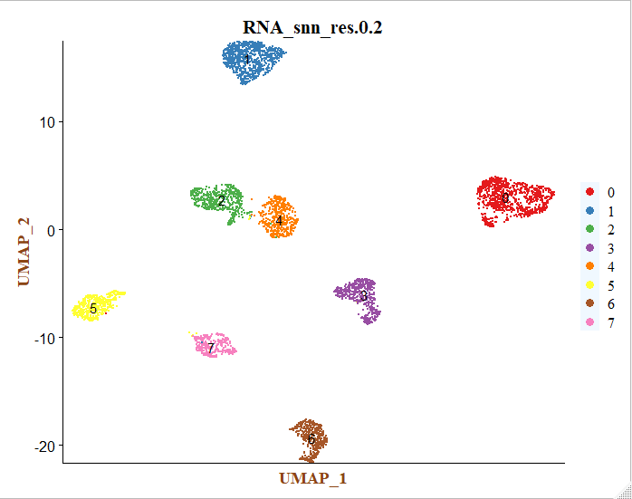
这个时候每个细胞亚群仅仅是顺序标号而已,后面需要进行生物学注释。
step3: 细胞亚群的生物学注释
根据之前的教程:混合到同一个10X样品里面的多个细胞系如何注释 可以获得与每个簇对应的细胞系,之后进行手动注释;
# cluster0 MCF7
# cluster1 HEK293
# cluster2 T47D
# cluster3 BCK4 # 排除法
# cluster4 T47D
# cluster5 MCF10A
# cluster6 MM134
# cluster7 SUM44

celltype <- data.frame(ClusterID = 0:7,
 celltype = c("MCF7","HEK293T","T47D WT","BCK4","T47D KO","MCF10A","MM134","SUM44"))
sce@meta.data$celltype_rep = "NA"
for(i in 1:nrow(celltype)){
 sce@meta.data[which(sce@meta.data$RNA_snn_res.0.2 == celltype$ClusterID[i])
 ,'celltype_rep'] <- celltype$celltype[i]}
#umap展示
colors <- c('#e41a1c','#377eb8','#4daf4a','#984ea3','#ff7f00','#ffff33','#a65628','#f781bf')
names(colors) <- unique(sce@meta.data$celltype_rep)

p_rep <- DimPlot(sce, reduction = "umap", group.by = "celltype_rep", label = T, cols = colors) +
 scale_y_continuous(expand = c(0, 0)) +
 scale_x_discrete(position = "bottom") +
 scale_fill_manual( breaks = rev(names(colors)),values = colors) +
 theme(
 plot.title = element_text(family = "serif", hjust = 0.5, vjust = 0, colour = "black"),
 # 坐标轴标题
 axis.title.x = element_text(family = "serif",face = "bold",colour = "chocolate4", hjust = 0.5, vjust = 0),
 axis.title.y = element_text(family = "serif",face = "bold",colour = "chocolate4", hjust = 0.5, vjust = 0.5),
 # # 坐标轴刻度
 # axis.text.x = element_text(family = "Yahei", vjust = 0.5, angle = 45),
 # axis.text.y = element_text(family = "Yahei" ),
 # axis.ticks = element_line(colour = "gray0", size = 0.9, linetype = "blank"),
 # 图例
 legend.title = element_text(hjust = 0.55,face = "bold", colour = "chocolate4",family = "serif"),
 legend.direction = "vertical",
 legend.text = element_text(family = "serif"),
 legend.key = element_rect(fill = "aliceblue"),
 legend.background = element_blank()
 )
p_rep
注释,根据文献里面的基因,检查每个细胞亚群的marker基因:
genes_in_paper <- c("BCAS3","PSMD6", "CSDE1", "RBP7" ,"TP53I3" ,"SERPINA6" ,
 "GNG11" ,"CLEC2B" ,"AZGP1" ,"CCND1", "AAMDC" ,"RSF1", "CNN3", "ARHGAP29" ,"LAPTM4A" ,
 "SCGB1D2" ,"SCGB2A2" ,"S100A1","KRT81", "KRT17", "KRT6A", "CKB","LDHB","RPL5")
colnames(sce@meta.data)
sce@meta.data$testclass <- factor(sce@meta.data$celltype_rep,
 levels = rev(c("MCF7","T47D WT","T47D KO","MM134",
 "SUM44","BCK4","MCF10A","HEK293T")))
Idents(sce)=sce$testclass
str(Idents(sce))

library(ggplot2)
p <- DotPlot(sce, assay = "RNA", features = genes_in_paper, cols = c("#bababa", "#ca0020"),)+
 #scale_y_continuous(expand = c(0, 0)) +
 scale_x_discrete(position = "bottom") +
 scale_fill_manual( breaks = rev(names(colors)),values = colors) +
 theme(plot.margin=margin(t = 0, b = 0, unit="pt"),
 plot.subtitle = element_text(family = "serif", colour = "gray0"),
 #plot.background = element_rect(fill = "aliceblue"),
 plot.title = element_text(face = "bold", family = "serif", hjust = 0.5, vjust = 0, colour = "black"),
 # 背景板
 panel.grid.minor = element_blank(),
 panel.grid.major.y = element_blank(),
 panel.background = element_blank(),
 # 坐标轴标题
 axis.title.x = element_text(family = "serif",face = "bold",colour = "chocolate4", hjust = 0.5, vjust = 0),
 axis.title.y = element_text(family = "serif",face = "bold",colour = "chocolate4", hjust = 0.5, vjust = 0.5),
 # 坐标轴刻度
 axis.text.x = element_text(family = "serif", vjust = 0.5, angle = 90),
 axis.text.y = element_text(family = "serif" ),
 axis.ticks = element_line(colour = "gray0", size = 0.9, linetype = "blank"),
 # 图例
 legend.title = element_text(hjust = 0.55,face = "bold", colour = "chocolate4",family = "serif"),
 legend.direction = "vertical",
 legend.text = element_text(family = "serif"),
 legend.key = element_rect(fill = "aliceblue"),
 #legend.background = element_rect(fill = "aliceblue")
 )
p
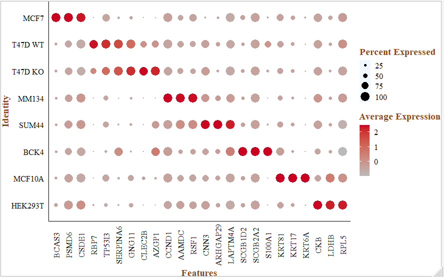
这样就完成了 《Single-Cell Transcriptomic Heterogeneity in Invasive Ductal and Lobular Breast Cancer Cells》这个文献里面的降维聚类分群和生物学注释图表。