gsea分析这方面教程我在《生信技能树》公众号写了不少了,不管是芯片还是测序的表达矩阵,都是一样的,把基因排序即可。那在单细胞分析里面也是如此,首先对指定的单细胞亚群可以做差异分析,然后就有了基因排序,后面gsea分析全部的代码无需修改,我这里演示一个简单的例子给大家哈!
安装seurat-data包获取测试数据
代码其实一句话即可:
devtools::install_github('satijalab/seurat-data')
但是因为是在GitHub,所以中国大陆地区的小伙伴有时候会遇到:
> devtools::install_github('satijalab/seurat-data')
Error: Failed to install 'SeuratData' from GitHub:
 Timeout was reached: [api.github.com] Operation timed out after 10002 milliseconds with 0 out of 0 bytes received
正常情况下应该是:
* installing *source* package ‘SeuratData’ ...
** using staged installation
** R
** exec
** inst
** byte-compile and prepare package for lazy loading
** help
*** installing help indices
** building package indices
** testing if installed package can be loaded from temporary location
** testing if installed package can be loaded from final location
** testing if installed package keeps a record of temporary installation path
* DONE (SeuratData)
查看以及认识测试数据
library(SeuratData)
AvailableData()
InstallData("pbmc3k") # (89.4 MB)
# trying URL 'http://seurat.nygenome.org/src/contrib/pbmc3k.SeuratData_3.1.4.tar.gz'
# 上面的 InstallData 代码只需要运行一次即可哈
data("pbmc3k")
exp <- pbmc3k@assays$RNA@data
dim(exp)
exp[1:4,1:4]
table(is.na(pbmc3k$seurat_annotations ))
这个测试数据pbmc3k,是已经做好了降维聚类分群和注释啦,这个数据集超级出名的,大家可以自行去了解它的背景知识哈。不幸的是元旦节假期我在中国大陆,所以这个下载简直是可怕
> InstallData("pbmc3k") # (89.4 MB)
trying URL 'http://seurat.nygenome.org/src/contrib/pbmc3k.SeuratData_3.1.4.tar.gz'
Content type 'application/octet-stream' length 93780025 bytes (89.4 MB)

downloaded 55 KB

Error in download.file(url, destfile, method, mode = "wb", ...) :
 download from 'http://seurat.nygenome.org/src/contrib/pbmc3k.SeuratData_3.1.4.tar.gz' failed
In addition: Warning messages:
1: In download.file(url, destfile, method, mode = "wb", ...) :
 downloaded length 56996 != reported length 93780025
2: In download.file(url, destfile, method, mode = "wb", ...) :
 URL 'https://seurat.nygenome.org/src/contrib/pbmc3k.SeuratData_3.1.4.tar.gz': status was 'Failure when receiving data from the peer'
虽然这个数据集失败了,我还有后手!
另外一个例子
可以看看我们前面的例子:人人都能学会的单细胞聚类分群注释 , 你必须要理解这个例子里面的降维聚类分群和注释。前面的seurat-data包的测试数据pbmc3k就是我们这个例子里面的 sce
rm(list=ls())
options(stringsAsFactors = F)
library(Seurat)
load(file = 'last_sce.Rdata')
sce
如下所示:
> exp <- sce@assays$RNA@data
> dim(exp)
[1] 19349 33168
> exp[1:4,1:4]
4 x 4 sparse Matrix of class "dgCMatrix"
 AAACCTGAGAGTAATC_1 AAACCTGGTAAATGTG_1 AAACGGGAGAAACGAG_1 AAACGGGAGGAGTACC_1
Sox17 1.663735 . . 1.916002
Mrpl15 . . . .
Lypla1 . . . .
Tcea1 . . . .
> table( sce$singleR )

B cells Endothelial cells Fibroblasts Fibroblasts activated
 4034 10578 94 309
 Hepatocytes Macrophages Monocytes NK cells
 1563 5105 4428 1180
 T cells
 5877
可以看到这个数据集是小鼠的哈,后面我们为了简单一点,直接采用把小鼠基因名字直接大写的方式,来转化为人类基因名字哦。
我们后面的分析也针对这个例子:人人都能学会的单细胞聚类分群注释 的数据吧。
针对指定的群做差异分析
我看了看,绝大部分都是免疫细胞,都被研究的太多了,比如我们看T细胞和B细胞的差异,应该是没有太大意思了。所以我就看看 Fibroblasts 和 Fibroblasts activated 这两个单细胞亚群吧,反正细胞数量也少,94个细胞对比309给,运算起来也很快哈。
指定亚群做单细胞分析,代码如下;
Idents(sce)='singleR'
deg=FindMarkers(object = sce, ident.1 = 'Fibroblasts',ident.2 = 'Fibroblasts activated',
 min.pct = 0.01, logfc.threshold = 0.01,
 thresh.use = 0.99)
head(deg)
批量做gsea分析
在msigdb数据库网页可以下载全部的基因集,我这里方便起见,仅仅是下载 h.all.v7.2.symbols.gmt文件:
### 对 MsigDB中的全部基因集 做GSEA分析。
# http://www.bio-info-trainee.com/2105.html
# http://www.bio-info-trainee.com/2102.html
# https://www.gsea-msigdb.org/gsea/msigdb
# https://www.gsea-msigdb.org/gsea/msigdb/collections.jsp
{
geneList= deg$avg_logFC
names(geneList)= toupper(rownames(deg))
geneList=sort(geneList,decreasing = T)
head(geneList)
library(ggplot2)
library(clusterProfiler)
library(org.Hs.eg.db)
#选择gmt文件(MigDB中的全部基因集)
gmtfile ='MSigDB/symbols/h.all.v7.2.symbols.gmt'
# 31120 个基因集
#GSEA分析
library(GSEABase) # BiocManager::install('GSEABase')
geneset <- read.gmt( gmtfile )
length(unique(geneset$term))
egmt <- GSEA(geneList, TERM2GENE=geneset,
minGSSize = 1,
pvalueCutoff = 0.99,
verbose=FALSE)
head(egmt)
egmt@result
gsea_results_df <- egmt@result
rownames(gsea_results_df)
write.csv(gsea_results_df,file = 'gsea_results_df.csv')
library(enrichplot)
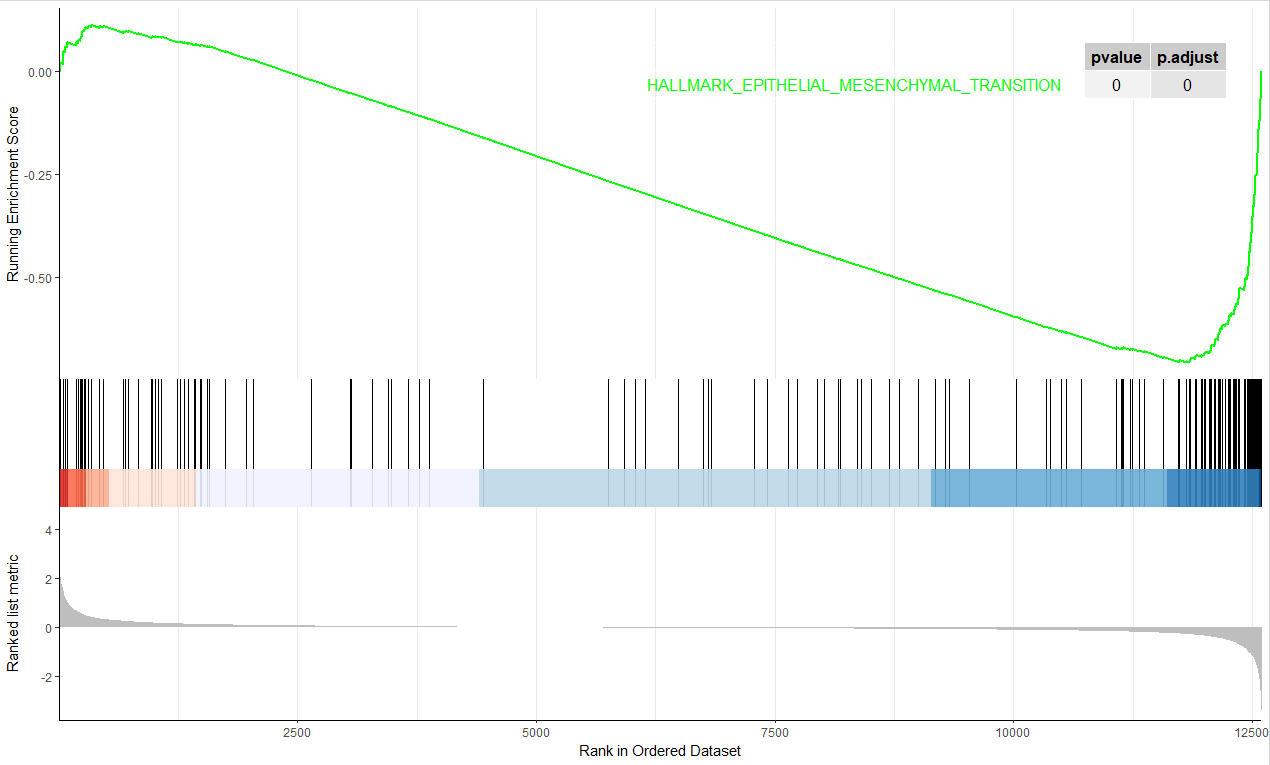
gseaplot2(egmt,geneSetID = 'HALLMARK_EPITHELIAL_MESENCHYMAL_TRANSITION',pvalue_table=T)
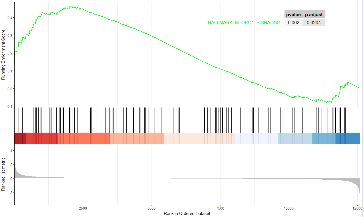
gseaplot2(egmt,geneSetID = 'HALLMARK_MTORC1_SIGNALING',pvalue_table=T)
}
得到的差异分析结果表格如下:
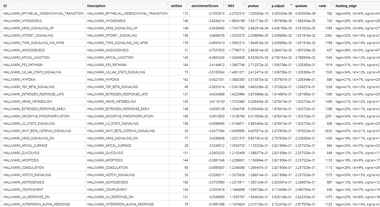
这个时候大家需要对Hallmark的50个基因集有一定的生物学认知,否则就只能是看数据本身了。
绘制其中一个上调通路如下:
绘制其中一个下调通路如下:
有意思的地方来了,为什么Fibroblasts 和 Fibroblasts activated 这两个单细胞亚群有这些通路的差异呢?这个生物学故事该如何去讲呢?这难道不是一篇文章吗?
把全部的基因集的gsea分析结果批量出图
假如你觉得我前面的代码很厉害,那么你可以考虑付费学习我下面的代码,收费3块钱:,会更厉害哦!
# 这里找不到显著下调的通路,可以选择调整阈值,或者其它。

down_kegg<-gsea_results_df[gsea_results_df$pvalue<0.05 & gsea_results_df$enrichmentScore < -0.3,];down_kegg$group=-1
up_kegg<-gsea_results_df[gsea_results_df$pvalue<0.05 & gsea_results_df$enrichmentScore > 0.3,];up_kegg$group=1

pro='test'
library(enrichplot)
lapply(1:nrow(down_kegg), function(i){
 gseaplot2(egmt,down_kegg$ID[i],
 title=down_kegg$Description[i],pvalue_table = T)
 ggsave(paste0(pro,'_down_kegg_',
 gsub('/','-',down_kegg$Description[i])
 ,'.pdf'))
})
lapply(1:nrow(up_kegg), function(i){
 gseaplot2(egmt,up_kegg$ID[i],
 title=up_kegg$Description[i],pvalue_table = T)
 ggsave(paste0(pro,'_up_kegg_',
 gsub('/','-',up_kegg$Description[i]),
 '.pdf'))
})
确实挺厉害的,如果你使用的是全部的msigdb数据库,可以出几百张图:
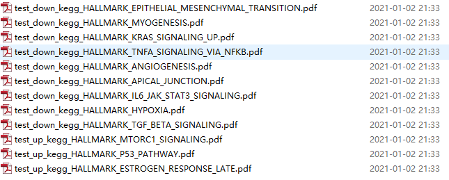
当然了,出图的名字可以去掉kegg这个数据库名字,因为我使用的hallmark哈。pathway在我这里是基因集的别名,其中msigdb数据库网页里面有着丰富的基因集,MSigDB(Molecular Signatures Database)数据库中定义了已知的基因集合:http://software.broadinstitute.org/gsea/msigdb 包括H和C1-C7八个系列(Collection),每个系列分别是:
- H: hallmark gene sets (癌症)特征基因集合,共50组,最常用;
- C1: positional gene sets 位置基因集合,根据染色体位置,共326个,用的很少;
- C2: curated gene sets:(专家)校验基因集合,基于通路、文献等:
- C3: motif gene sets:模式基因集合,主要包括microRNA和转录因子靶基因两部分
- C4: computational gene sets:计算基因集合,通过挖掘癌症相关芯片数据定义的基因集合;
- C5: GO gene sets:Gene Ontology 基因本体论,包括BP(生物学过程biological process,细胞原件cellular component和分子功能molecular function三部分)
- C6: oncogenic signatures:癌症特征基因集合,大部分来源于NCBI GEO 发表芯片数据
- C7: immunologic signatures: 免疫相关基因集合。
- 最近还新出来了一个单细胞的基因集哦,大家可以去看看
可以试试看iDEA这个网页工具哦
University of Michigan的课题组于2020年3月发表在NC杂志的文章:《Integrative differential expression and gene set enrichment analysis using summary statistics for scRNA-seq studies》,链接是:https://www.nature.com/articles/s41467-020-15298-6
- Differential expression (DE) analysis and gene set enrichment (GSE) analysis are commonly applied in single cell RNA sequencing (scRNA-seq) studies.
- Here, we develop an integrative and scalable computational method, iDEA, to perform joint DE and GSE analysis through a hierarchical Bayesian framework.
- By integrating DE and GSE analyses, iDEA can improve the power and consistency of DE analysis and the accuracy of GSE analysis.
比如GSEA分析,我也多次讲解:
但实际上,绝大部分读者并没有去细看这个统计学原理,也不需要知道gsea分析的nes值如何计算