前面我们展现了 CNS图表复现08—肿瘤单细胞数据第一次分群通用规则,然后呢,第二次分群的上皮细胞可以细分恶性与否,免疫细胞呢,细分可以成为: B细胞,T细胞,巨噬细胞,树突细胞等等。实际上每个免疫细胞亚群仍然可以继续精细的划分,以文章为例:
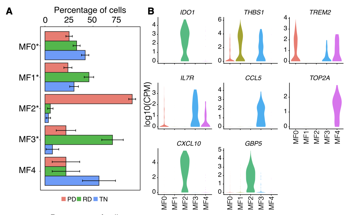
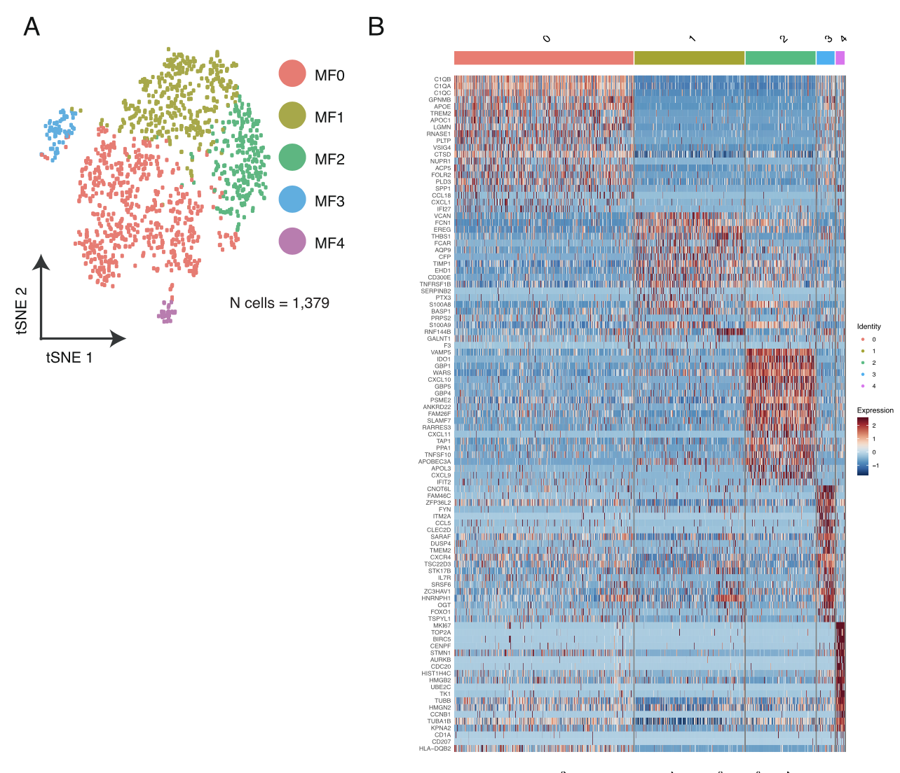
- Macrophages from lung tumor biopsies (n = 1,379) were clus- tered into 5 distinct groups (Figure S7A) followed by differential gene expression in each resulting cluster
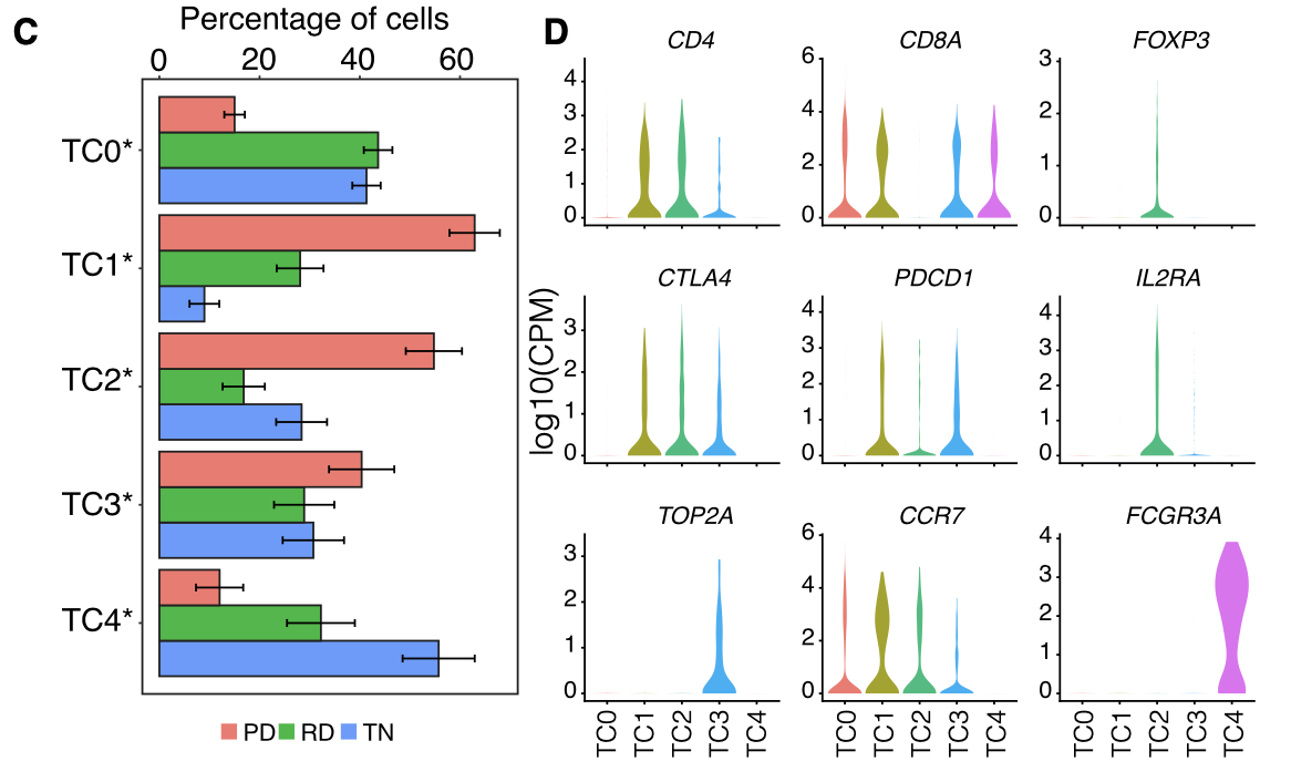
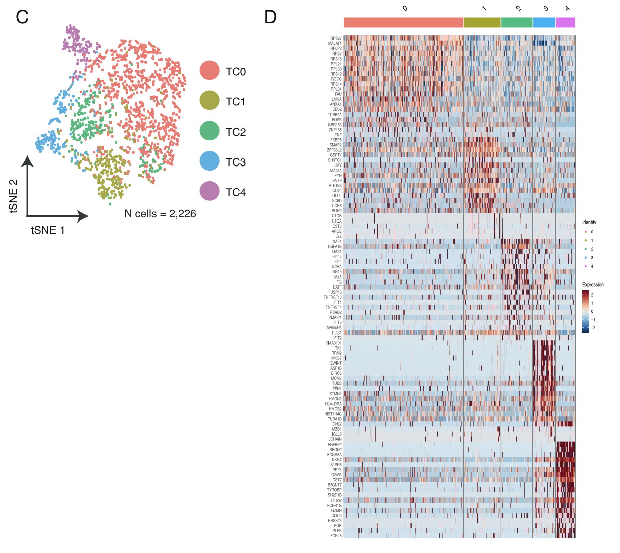
- T cells and NK cells (n = 2,226) were analyzed in the same manner as macrophages and resulted in 5 distinct T/NK cell pop- ulations .
这就是正文的图表5:
首先是Macrophages细分 :
各个细胞亚群的比例展示及标记基因小提琴图:
各个细胞亚群的分布情况及标记基因热图;
然后是T cells and NK cells的细分
各个细胞亚群的比例展示及标记基因小提琴图:
各个细胞亚群的分布情况及标记基因热图;
尝试复现T细胞的亚群细分
文章提到的是
- Macrophages from lung tumor biopsies (n = 1,379) were clus- tered into 5 distinct groups (Figure S7A) followed by differential gene expression in each resulting cluster
- T cells and NK cells (n = 2,226) were analyzed in the same manner as macrophages and resulted in 5 distinct T/NK cell pop- ulations .
首先我们拿到T cells and NK cells数据集
rm(list=ls())
options(stringsAsFactors = F)
library(Seurat)
library(ggplot2)
### 来源于:CNS图表复现02—Seurat标准流程之聚类分群的step1-create-sce.R
load(file = 'first_sce.Rdata')

### 来源于 step2-anno-first.R
load(file = 'phe-of-first-anno.Rdata')

sce=sce.first
table(phe$immune_annotation)
# # immune (CD45+,PTPRC), epithelial/cancer (EpCAM+,EPCAM), and stromal (CD10+,MME,fibo or CD31+,PECAM1,endo)

genes_to_check = c("PTPRC","CD19",'PECAM1','MME','CD3G', 'CD4', 'CD8A' )
p <- DotPlot(sce, features = genes_to_check,
 assay='RNA' )
p
table(phe$immune_annotation,phe$seurat_clusters)

cells.use <- row.names(sce@meta.data)[which(phe$immune_annotation=='immune')]
length(cells.use)
sce <-subset(sce, cells=cells.use)
sce

# 实际上这里需要重新对sce进行降维聚类分群,为了节省时间
# 我们直接载入前面的降维聚类分群结果,但是并没有载入tSNE哦
## 来源于: CNS图表复现05—免疫细胞亚群再分类
load(file = 'phe-of-subtypes-Immune-by-manual.Rdata')
sce@meta.data=phe
table(phe$immuSub)

# 需要背景知识
# https://www.abcam.com/primary-antibodies/immune-cell-markers-poster
# NK Cell* CD11b+, CD122+, NK1.1+, NKG2D+, NKp46+
# NCR1 Gene. Natural Cytotoxicity Triggering Receptor 1; NK-P46; Natural Killer Cell P46-Related Protein;
# NKG2D is a transmembrane protein belonging to the NKG2 family of C-type lectin-like receptors. NKG2D is encoded by KLRK1 gene

# T Cell* CD3+
genes_to_check = c('CD3G', 'CD4', 'CD8A', 'FOXP3',
 'TNF','IFNG','KLRK1','NCR1')
p <- DotPlot(sce, features = genes_to_check,group.by = 'seurat_clusters') + coord_flip()
p

cells.use <- row.names(sce@meta.data)[which(phe$immuSub=='Tcells')]
length(cells.use)
sce <-subset(sce, cells=cells.use)
sce
# 26485 features across 4555 samples within 1 assay
然后走降维聚类分群流程
挑选出来了 4555 个细胞,走标准流程即可:
sce <- NormalizeData(sce, normalization.method = "LogNormalize",
 scale.factor = 10000)
GetAssay(sce,assay = "RNA")
sce <- FindVariableFeatures(sce,
 selection.method = "vst", nfeatures = 2000)
# 步骤 ScaleData 的耗时取决于电脑系统配置(保守估计大于一分钟)
sce <- ScaleData(sce)
sce <- RunPCA(object = sce, pc.genes = VariableFeatures(sce))
DimHeatmap(sce, dims = 1:12, cells = 100, balanced = TRUE)
ElbowPlot(sce)
sce <- FindNeighbors(sce, dims = 1:15)
sce <- FindClusters(sce, resolution = 0.2)
table(sce@meta.data$RNA_snn_res.0.2)
sce <- RunUMAP(object = sce, dims = 1:15, do.fast = TRUE)
DimPlot(sce,reduction = "umap",label=T)
# 这个时候分成了6群
查亚群的标记基因
如果我们去 https://www.abcam.com/primary-antibodies/t-cells-basic-immunophenotyping 可以看到
- Killer T cells (cytotoxic T lymphocytes: CD8+) , Effector or memory
- Helper T cells (Th cells: CD4+), TH1,2,17
- Regulatory T cells (Treg cells: CD4+, CD25+, FoxP3+, CD127+)
- interferon gamma (IFN-γ) and tumor necrosis factor alpha (TNF-α), two factors produced by activated T cells
- Helper Th1,IFNγ, IL-2, IL-12, IL-18
比较简单的CD4,CD8,以及FOXP3各自代表的T细胞亚群。比较复杂的可以是:张泽民团队的单细胞研究把T细胞分的如此清楚
但是很不幸,在这个数据集里面它们都不是主要的细胞亚群决定因素。
genes_to_check = c('CD3G', 'CD4', 'CD8A', 'FOXP3',
 'TNF','IFNG','KLRK1','NCR1')
p1 <- DotPlot(sce, features = genes_to_check,group.by = 'seurat_clusters') + coord_flip()
p1
p2=DimPlot(sce,reduction = "umap",label=T)
library(patchwork)
p1+p2
出图如下:
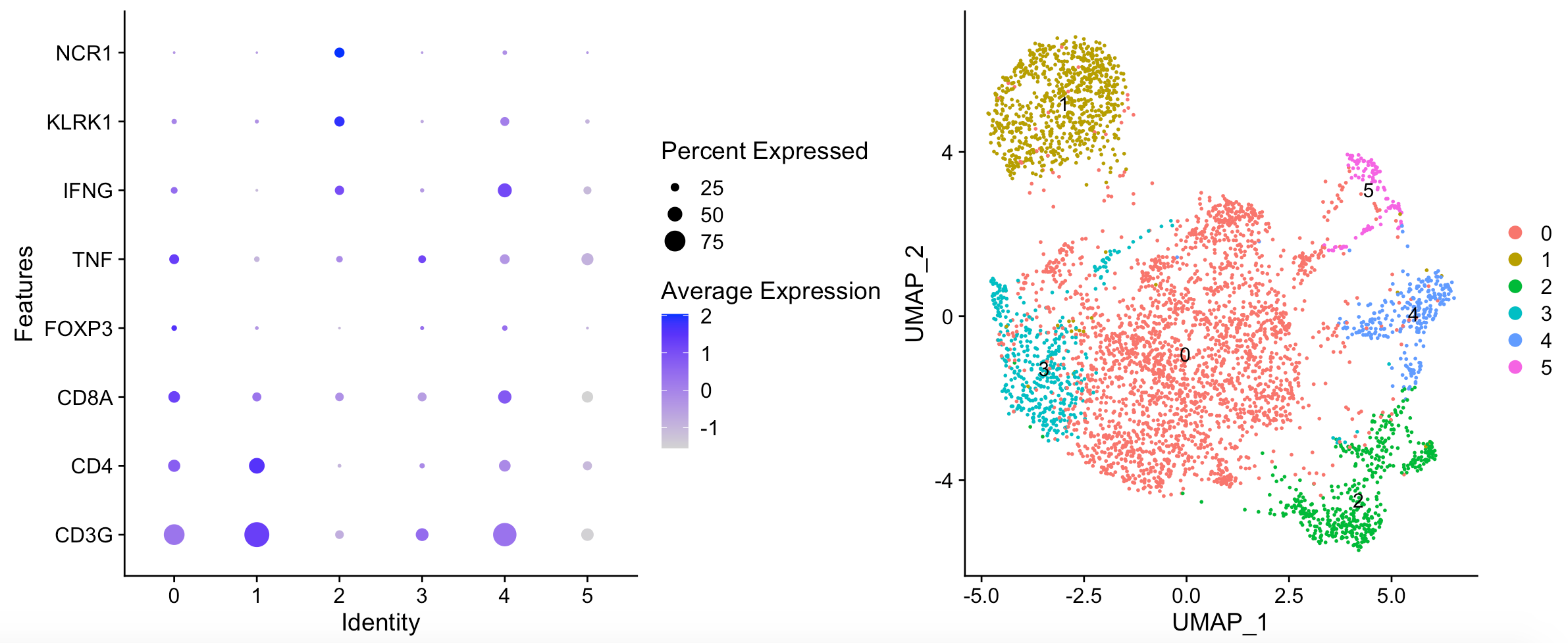
文章呢,选取的其实是 biopsy_site == “Lung” 的T cells and NK cells (n = 2,226) ,区分成为5 distinct T/NK cell pop- ulations .
> table(sce@meta.data$biopsy_site)

Adrenal Brain Liver LN lung Lung Pleura
 226 2 586 700 485 1692 864
所以我们只能是继续挑选子集走流程。代码如下:
sce <- NormalizeData(sce, normalization.method = "LogNormalize",
 scale.factor = 10000)
GetAssay(sce,assay = "RNA")
sce <- FindVariableFeatures(sce,
 selection.method = "vst", nfeatures = 2000)
# 步骤 ScaleData 的耗时取决于电脑系统配置(保守估计大于一分钟)
sce <- ScaleData(sce)
sce <- RunPCA(object = sce, pc.genes = VariableFeatures(sce))
DimHeatmap(sce, dims = 1:12, cells = 100, balanced = TRUE)
ElbowPlot(sce)
sce <- FindNeighbors(sce, dims = 1:15)
sce <- FindClusters(sce, resolution = 0.5)
table(sce@meta.data$RNA_snn_res.0.5)
sce <- RunUMAP(object = sce, dims = 1:15, do.fast = TRUE)
genes_to_check = c('CD3G', 'CD4', 'CD8A', 'FOXP3',
 'TNF','IFNG','KLRK1','NCR1')
p1 <- DotPlot(sce, features = genes_to_check,group.by = 'seurat_clusters') + coord_flip()
p1
p2=DimPlot(sce,reduction = "umap",label=T)
library(patchwork)
p1+p2
可以看到,并没有本质上的区别:
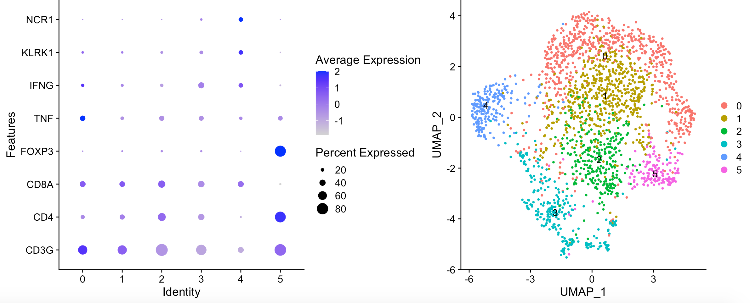
复现失败了!唯一看起来比较类似的就是 FOXP3 positive Tregs in cluster 5,哈哈哈哈!
- Cluster0: generic dont really know.
- Cluster1: Exhaustion in the pD cluster (1) and the PD/PR cluster (4). (PR/PD feature)
- Cluster2: Cluster 2 is cytotoxic (GZMK, EOMES, CD8pos, IFNG) (Less in PD)
- Cluster3: Cluster 3 is enriched for NK cells (Naive feature)
- Cluster4: Exhaustion in the pD cluster (1) and the PD/PR cluster (4). (PR/PD feature)
- Cluster5: FOXP3 positive Tregs in cluster 5 (Less in PR)
往期教程目录:
- CNS图表复现01—读入csv文件的表达矩阵构建Seurat对象
- CNS图表复现02—Seurat标准流程之聚类分群
- CNS图表复现03—单细胞区分免疫细胞和肿瘤细胞
- CNS图表复现04—单细胞聚类分群的resolution参数问题
- CNS图表复现05—免疫细胞亚群再分类
- CNS图表复现06—根据CellMarker网站进行人工校验免疫细胞亚群
- CNS图表复现07—原来这篇文章有两个单细胞表达矩阵
- CNS图表复现08—肿瘤单细胞数据第一次分群通用规则
- CNS图表复现09—上皮细胞可以区分为恶性与否
- CNS图表复现10—表达矩阵是如何得到的
- CNS图表复现11—RNA-seq数据可不只是表达量矩阵结果
- CNS图表复现12—检查原文的细胞亚群的标记基因
- CNS图表复现13—使用inferCNV来区分肿瘤细胞的恶性与否
- CNS图表复现14—检查文献的inferCNV流程
- CNS图表复现15—inferCNV流程输入数据差异大揭秘
- CNS图表复现16—inferCNV结果解读及利用
- CNS图表复现17—inferCNV结果解读及利用之进阶