数据挖掘的本质是把基因数量搞小,比如表达量矩阵通常是2万多个蛋白编码基因,不管是表达芯片还是RNA-seq测序的,采用何种程度的差异分析,最后都还有成百上千个目标基因。如果是临床队列,通常是会跟生存分析进行交集,或者多个数据集差异结果的交集,比如:多个数据集整合神器-RobustRankAggreg包 ,这样的基因集就是100个以内的数量了,但是仍然有缩小的空间,比如lasso等统计学算法,最后搞成10个左右的基因组成signature即可顺利发表。
但是lasso等统计学算法对绝大部分半路出家的数据分析师来说,想从原理到操作全部吃透还是有一点困难的。这里我推荐一个R包 glmSparseNet,可以完成多种数据类型的lasso回归,包括:”gaussian”, “poisson”, “binomial”, “multinomial”, “cox”, and “mgaussian”.
这个包的全称是:Network Centrality Metrics for Elastic-Net Regularized Models,官网是:https://www.bioconductor.org/packages/release/bioc/html/glmSparseNet.html 给出了多个实例文档,非常值得读完:
HTML R Script Breast survival dataset using network from STRING DB
HTML R Script Example for Classification -- Breast Invasive Carcinoma
HTML R Script Example for Survival Data -- Breast Invasive Carcinoma
HTML R Script Example for Survival Data -- Prostate Adenocarcinoma
HTML R Script Example for Survival Data -- Skin Melanoma
安装和加载R包glmSparseNet的方法相信已经无需我多说了:
if (!require("BiocManager"))
 install.packages("BiocManager")
BiocManager::install("glmSparseNet")
3个癌症数据的例子
这里使用 curatedTCGAData 来获取TCGA数据库的数据,参考教程:使用curatedTCGAData下载TCGA数据库信息好用吗,首先带领大家认识一下这些数据。
首先是乳腺癌
如果是分类模型构建,区分肿瘤样品和正常组织的表达量样品,获取数据的代码如下:
library(curatedTCGAData)
library(TCGAutils)
params <- list(seed = 29221)

brca <- curatedTCGAData(diseaseCode = "BRCA", assays = "RNASeq2GeneNorm", FALSE)
## ----data.show, warning=FALSE, error=FALSE------------------------------------
brca <- TCGAutils::splitAssays(brca, c('01','11'))
xdata.raw <- t(cbind(assay(brca[[1]]), assay(brca[[2]])))

# Get matches between survival and assay data
class.v <- TCGAbiospec(rownames(xdata.raw))$sample_definition %>% factor
names(class.v) <- rownames(xdata.raw)
# keep features with standard deviation > 0
xdata.raw <- xdata.raw %>%
 { (apply(., 2, sd) != 0) } %>%
 { xdata.raw[, .] } %>%
 scale

set.seed(params$seed)
small.subset <- c('CD5', 'CSF2RB', 'HSF1', 'IRGC', 'LRRC37A6P', 'NEUROG2',
 'NLRC4', 'PDE11A', 'PIK3CB', 'QARS', 'RPGRIP1L', 'SDC1',
 'TMEM31', 'YME1L1', 'ZBTB11',
 sample(colnames(xdata.raw), 100))

xdata <- xdata.raw[, small.subset[small.subset %in% colnames(xdata.raw)]]
ydata <- class.v
save(xdata,ydata,file = 'brca_for_lasso.rdata')

# 可以看到 肿瘤样品大概是正常样品的10倍数量。
> table(ydata)
ydata
Primary Solid Tumor Solid Tissue Normal
 1093 112
如果是生存分析模型构建,需要的数据是纯粹的肿瘤样品表达矩阵加上对应的肿瘤病人的生存信息,全部下载的代码如下:
params <- list(seed = 29221)

brca <- curatedTCGAData(diseaseCode = "BRCA", assays = "RNASeq2GeneNorm", FALSE)
brca.primary.solid.tumor <- TCGAutils::splitAssays(brca, '01')
xdata.raw <- t(assay(brca.primary.solid.tumor[[1]]))

# Get survival information
ydata.raw <- colData(brca.primary.solid.tumor) %>% as.data.frame %>%
 # Keep only data relative to survival or samples
 select(patientID, vital_status,
 Days.to.date.of.Death, Days.to.Date.of.Last.Contact,
 days_to_death, days_to_last_followup,
 Vital.Status) %>%
 # Convert days to integer
 mutate(Days.to.date.of.Death = as.integer(Days.to.date.of.Death)) %>%
 mutate(Days.to.Last.Contact = as.integer(Days.to.Date.of.Last.Contact)) %>%
 # Find max time between all days (ignoring missings)
 rowwise %>%
 mutate(time = max(days_to_last_followup, Days.to.date.of.Death,
 Days.to.Last.Contact, days_to_death, na.rm = TRUE)) %>%
 # Keep only survival variables and codes
 select(patientID, status = vital_status, time) %>%
 # Discard individuals with survival time less or equal to 0
 filter(!is.na(time) & time > 0) %>% as.data.frame

# Set index as the patientID
rownames(ydata.raw) <- ydata.raw$patientID

# Get matches between survival and assay data
xdata.raw <- xdata.raw[TCGAbarcode(rownames(xdata.raw)) %in%
 rownames(ydata.raw),]
xdata.raw <- xdata.raw %>%
 { (apply(., 2, sd) != 0) } %>%
 { xdata.raw[, .] } %>%
 scale

# Order ydata the same as assay
ydata.raw <- ydata.raw[TCGAbarcode(rownames(xdata.raw)), ]

# Using only a subset of genes previously selected to keep this short example.
set.seed(params$seed)
small.subset <- c('CD5', 'CSF2RB', 'IRGC', 'NEUROG2', 'NLRC4', 'PDE11A',
 'PTEN', 'TP53', 'BRAF',
 'PIK3CB', 'QARS', 'RFC3', 'RPGRIP1L', 'SDC1', 'TMEM31',
 'YME1L1', 'ZBTB11', sample(colnames(xdata.raw), 100)) %>%
 unique

xdata <- xdata.raw[, small.subset[small.subset %in% colnames(xdata.raw)]]
ydata <- ydata.raw %>% select(time, status)
save(xdata,ydata,file = 'brca_for_lasso_sur.rdata')

> head(ydata)
 time status
TCGA-3C-AAAU 4047 0
TCGA-3C-AALI 4005 0
TCGA-3C-AALJ 1474 0
TCGA-3C-AALK 1448 0
TCGA-4H-AAAK 348 0
TCGA-5L-AAT0 1477 0
可以看到,虽然变量名都是 ydata ,但是里面存储的数据不一样哦。
然后是前列腺癌
代码如下:
library(curatedTCGAData)
library(TCGAutils)
params <- list(seed = 29221)

prad <- curatedTCGAData(diseaseCode = "PRAD", assays = "RNASeq2GeneNorm", FALSE)
prad.primary.solid.tumor <- TCGAutils::splitAssays(prad, '01')
xdata.raw <- t(assay(prad.primary.solid.tumor[[1]]))

# Get survival information
ydata.raw <- colData(prad.primary.solid.tumor) %>% as.data.frame %>%
 # Find max time between all days (ignoring missings)
 rowwise %>%
 mutate(time = max(days_to_last_followup, days_to_death, na.rm = TRUE)) %>%
 # Keep only survival variables and codes
 select(patientID, status = vital_status, time) %>%
 # Discard individuals with survival time less or equal to 0
 filter(!is.na(time) & time > 0) %>% as.data.frame

# Set index as the patientID
rownames(ydata.raw) <- ydata.raw$patientID

# keep only features that have standard deviation > 0
xdata.raw <- xdata.raw[TCGAbarcode(rownames(xdata.raw)) %in%
 rownames(ydata.raw),]
xdata.raw <- xdata.raw %>%
 { (apply(., 2, sd) != 0) } %>%
 { xdata.raw[, .] } %>%
 scale

# Order ydata the same as assay
ydata.raw <- ydata.raw[TCGAbarcode(rownames(xdata.raw)), ]

set.seed(params$seed)
small.subset <- c(geneNames(c('ENSG00000103091', 'ENSG00000064787',
 'ENSG00000119915', 'ENSG00000120158',
 'ENSG00000114491', 'ENSG00000204176',
 'ENSG00000138399'))$external_gene_name,
 sample(colnames(xdata.raw), 100)) %>% unique %>% sort

xdata <- xdata.raw[, small.subset[small.subset %in% colnames(xdata.raw)]]
ydata <- ydata.raw %>% select(time, status)
save(xdata,ydata,file = 'prad_for_lasso.rdata')
最后是皮肤癌
代码如下:
library(curatedTCGAData)
library(TCGAutils)
params <- list(seed = 29221)

skcm <- curatedTCGAData(diseaseCode = 'SKCM', assays = 'RNASeq2GeneNorm', FALSE, cache = tempdir())
skcm.metastatic <- TCGAutils::splitAssays(skcm, '06')
xdata.raw <- t(assay(skcm.metastatic[[1]]))
# Get survival information
ydata.raw <- colData(skcm.metastatic) %>% as.data.frame %>%
 # Find max time between all days (ignoring missings)
 rowwise %>%
 mutate(time = max(days_to_last_followup, days_to_death, na.rm = TRUE)) %>%
 # Keep only survival variables and codes
 select(patientID, status = vital_status, time) %>%
 # Discard individuals with survival time less or equal to 0
 filter(!is.na(time) & time > 0) %>% as.data.frame

# Get survival information
ydata.raw <- colData(skcm) %>% as.data.frame %>%
 # Find max time between all days (ignoring missings)
 rowwise %>%
 mutate(time = max(days_to_last_followup, days_to_death, na.rm = TRUE)) %>%
 # Keep only survival variables and codes
 select(patientID, status = vital_status, time) %>%
 # Discard individuals with survival time less or equal to 0
 filter(!is.na(time) & time > 0) %>% as.data.frame

# Set index as the patientID
rownames(ydata.raw) <- ydata.raw$patientID

# keep only features that have standard deviation > 0
xdata.raw <- xdata.raw[TCGAbarcode(rownames(xdata.raw)) %in%
 rownames(ydata.raw),]
xdata.raw <- xdata.raw %>%
 { (apply(., 2, sd) != 0) } %>%
 { xdata.raw[, .] } %>%
 scale

# Order ydata the same as assay
ydata.raw <- ydata.raw[TCGAbarcode(rownames(xdata.raw)), ]

set.seed(params$seed)
small.subset <- c('FOXL2', 'KLHL5', 'PCYT2', 'SLC6A10P', 'STRAP', 'TMEM33',
 'WT1-AS', sample(colnames(xdata.raw), 100))

xdata <- xdata.raw[, small.subset[small.subset %in% colnames(xdata.raw)]]
ydata <- ydata.raw %>% select(time, status)

save(xdata,ydata,file = 'skcm_for_lasso.rdata')
后面的建模就靠这些数据文件啦:

前面的数据下载,仅仅是准备工作,跟一句代码完成lasso回归没有关系哈。如果看不懂,自己再去翻教程:使用curatedTCGAData下载TCGA数据库信息好用吗,反正我给出来了的代码都是复制粘贴就可以运行的。
使用函数cv.glmHub来处理xdata和ydata即可进行lasso回归
如果ydata存的是肿瘤或者正常样品这样的属性,我们使用cv.glmHub来做分类模型构建,如果ydata存的是肿瘤生存信息,那么我们使用cv.glmHub来做生存分析的模型构建。
library(dplyr)
library(ggplot2)
library(survival)
library(loose.rock)
library(futile.logger)
library(curatedTCGAData)
library(TCGAutils)
library(glmSparseNet)
首先是分类模型构建
ydata存的是肿瘤或者正常样品这样的属性,是二分类,使用函数cv.glmHub 一句话代码即可完成分析:
load('brca_for_lasso.rdata')
table(ydata)
fitted <- cv.glmHub(xdata, ydata,
 family = 'binomial',
 network = 'correlation',
 nlambda = 1000,
 network.options = networkOptions(cutoff = .6,
 min.degree = .2))

plot(fitted)
resp <- predict(fitted, s = 'lambda.min', newx = xdata, type = 'class')
table(resp,ydata)
关键的参数是 family = ‘binomial’, 然后可以看到,这个分类器效果还不错:
> table(resp,ydata)
 ydata
resp Primary Solid Tumor Solid Tissue Normal
 Primary Solid Tumor 1088 11
 Solid Tissue Normal 5 101
基本上没有分错的样品。
当然了,还可以去提取构建好的分类器的主要基因,以及绘制ROC曲线等等,是另外的知识点了,这里仅仅是分享代码:
coefs.v <- coef(fitted, s = 'lambda.min')[,1] %>% { .[. != 0]}
coefs.v %>% {
 data.frame(ensembl.id = names(.),
 gene.name = geneNames(names(.))$external_gene_name,
 coefficient = .,
 stringsAsFactors = FALSE)
} %>%
 arrange(gene.name) %>%
 knitr::kable()

flog.info('Misclassified (%d)', sum(ydata != resp))
flog.info(' * False primary solid tumour: %d',
 sum(resp != ydata & resp == 'Primary Solid Tumor'))
flog.info(' * False normal : %d',
 sum(resp != ydata & resp == 'Solid Tissue Normal'))

## ----predict, echo=FALSE, warning=FALSE---------------------------------------
response <- predict(fitted, s = 'lambda.min', newx = xdata, type = 'response')
qplot(response, bins = 100)

## ----roc, echo=FALSE----------------------------------------------------------
roc_obj <- pROC::roc(ydata, as.vector(response))

data.frame(TPR = roc_obj$sensitivities, FPR = 1 - roc_obj$specificities) %>%
 ggplot() +geom_line(aes(FPR,TPR), color = 2, size = 1, alpha = 0.7)+
 labs(title= sprintf("ROC curve (AUC = %f)", pROC::auc(roc_obj)),
 x = "False Positive Rate (1-Specificity)",
 y = "True Positive Rate (Sensitivity)")
上面的代码都是复制粘贴就可以运行的。
然后是生存分析的模型构建
同样的,使用函数cv.glmHub一句话代码即可完成分析:
fitted <- cv.glmHub(xdata, Surv(ydata$time, ydata$status),
 family = 'cox',
 lambda = buildLambda(1),
 network = 'correlation',
 network.options = networkOptions(cutoff = .6,
 min.degree = .2))
plot(fitted)
注意,这个时候的参数 family = ‘cox’, 不过同样的,可以提取分类器的基因,看其对应的基因集,也不重要;
coefs.v <- coef(fitted, s = 'lambda.min')[,1] %>% { .[. != 0]}
coefs.v %>% {
 data.frame(gene.name = names(.),
 coefficient = .,
 stringsAsFactors = FALSE)
} %>%
 arrange(gene.name) %>%
 knitr::kable()

names(coefs.v) %>% { hallmarks(.)$heatmap }
lasso回归确定的基因是3个,如下:
| |gene.name | coefficient|
|:-----|:---------|-----------:|
|CD5 |CD5 | -0.1115553|
|RPS15 |RPS15 | -0.1266871|
|ZNF80 |ZNF80 | -0.0645328|

$km
Call: survfit(formula = survival::Surv(time, status) ~ group, data = prognostic.index.df)

n events median 0.95LCL 0.95UCL
Low risk 540 64 4456 3669 NA
High risk 540 88 3738 3126 NA

> coefs.v
 CD5 ZNF80 RPS15
-0.11155531 -0.06453279 -0.12668706
最重要的是我们构建好的生存预测模型的效果:
coefs.v
separate2GroupsCox(as.vector(coefs.v),
 xdata[, names(coefs.v)],
 ydata,
 plot.title = 'Full dataset', legend.outside = FALSE)
出图如下,还挺显著的:
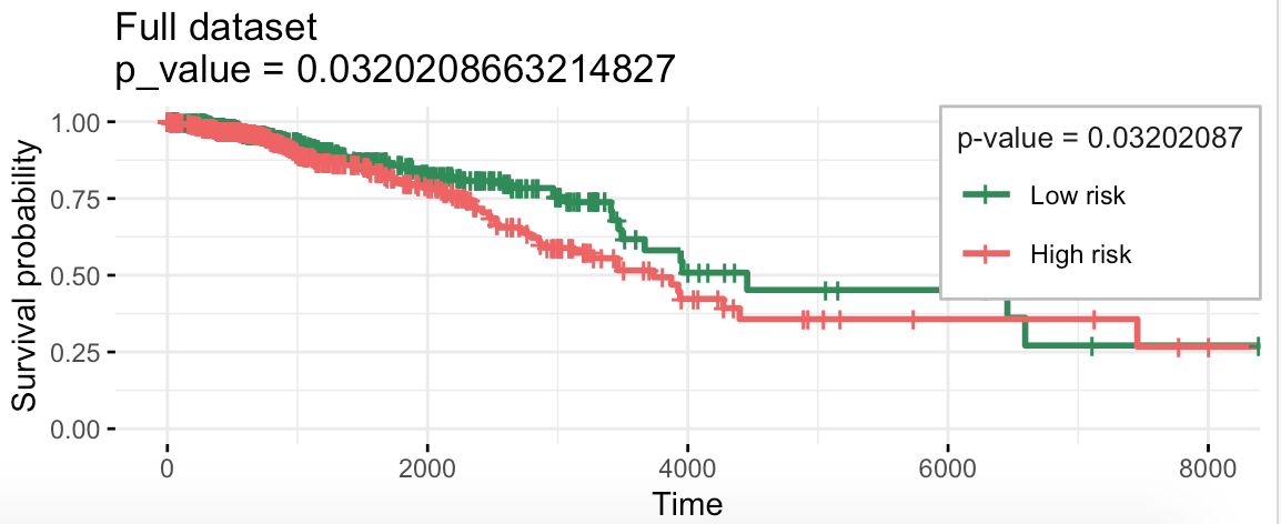
构建好的这个模型相关不错哦。
另外的两个数据集,大家自行去验证吧!
真实案例
前面的表达矩阵和表型信息,我们都是直接使用了教程:使用curatedTCGAData下载TCGA数据库信息好用吗,随机挑选的基因,所以我们设置好了随机数种子,params <- list(seed = 29221) 。不过真实情况下,我们的基因首先应该是被挑选过一次,一般来说是差异分析,或者wgcna分析,拿到的差异及列表或者某个模块的基因列表。数据集呢,通常是1000以内,然后去走lasso回归分析,定位到更少的基因数量。与我最开始点题的数据挖掘的本质是把基因数量搞小相呼应啦。
学徒作业
前面的TCGA数据库的BRCA数据集里面,可以挑选出来TNBC亚型的表达矩阵,约100个左右的样品,部分病人是有化疗信息的,把他们区分成为缓解组和没有效果的两个组,这样的话首先可以做一下差异分析拿到约1000个左右的差异基因。然后呢,针对这约1000个左右的差异基因的约100个左右的样品表达矩阵走我们的教程,一句代码完成lasso回归,看看构建好的模型预测化疗效果的能力!