上个月我们组建了:《单细胞CNS图表复现交流群》,见:你要的rmarkdown文献图表复现全套代码来了(单细胞),也分享了单细胞转录组数据分析的流程:
交流群里大家讨论的热火朝天,而且也都开始了图表复现之旅,在这里我还是带大家一步步学习CNS图表吧。如果你也想加入交流群,自己去:你要的rmarkdown文献图表复现全套代码来了(单细胞)找到我们的拉群小助手哈。
今天讲解第二步:完成Seurat标准流程之聚类分群。
直接上代码:
raw_sce <- main_tiss_filtered

raw_sce
rownames(raw_sce)[grepl('^mt-',rownames(raw_sce),ignore.case = T)]
rownames(raw_sce)[grepl('^Rp[sl]',rownames(raw_sce),ignore.case = T)]

raw_sce[["percent.mt"]] <- PercentageFeatureSet(raw_sce, pattern = "^MT-")
fivenum(raw_sce[["percent.mt"]][,1])
rb.genes <- rownames(raw_sce)[grep("^RP[SL]",rownames(raw_sce),ignore.case = T)]
C<-GetAssayData(object = raw_sce, slot = "counts")
percent.ribo <- Matrix::colSums(C[rb.genes,])/Matrix::colSums(C)*100
fivenum(percent.ribo)
raw_sce <- AddMetaData(raw_sce, percent.ribo, col.name = "percent.ribo")

plot1 <- FeatureScatter(raw_sce, feature1 = "nCount_RNA", feature2 = "percent.ercc")
plot2 <- FeatureScatter(raw_sce, feature1 = "nCount_RNA", feature2 = "nFeature_RNA")
CombinePlots(plots = list(plot1, plot2))

VlnPlot(raw_sce, features = c("percent.ribo", "percent.ercc"), ncol = 2)
VlnPlot(raw_sce, features = c("nFeature_RNA", "nCount_RNA"), ncol = 2)
VlnPlot(raw_sce, features = c("percent.ribo", "nCount_RNA"), ncol = 2)
raw_sce

sce=raw_sce
sce
sce <- NormalizeData(sce, normalization.method = "LogNormalize",
 scale.factor = 10000)
GetAssay(sce,assay = "RNA")
sce <- FindVariableFeatures(sce,
 selection.method = "vst", nfeatures = 2000)
# 步骤 ScaleData 的耗时取决于电脑系统配置(保守估计大于一分钟)
sce <- ScaleData(sce)
sce <- RunPCA(object = sce, pc.genes = VariableFeatures(sce))
DimHeatmap(sce, dims = 1:12, cells = 100, balanced = TRUE)
ElbowPlot(sce)
sce <- FindNeighbors(sce, dims = 1:15)
sce <- FindClusters(sce, resolution = 0.2)
table(sce@meta.data$RNA_snn_res.0.2)
sce <- FindClusters(sce, resolution = 0.8)
table(sce@meta.data$RNA_snn_res.0.8)

library(gplots)
tab.1=table(sce@meta.data$RNA_snn_res.0.2,sce@meta.data$RNA_snn_res.0.8)
balloonplot(tab.1)

set.seed(123)
sce <- RunTSNE(object = sce, dims = 1:15, do.fast = TRUE)
DimPlot(sce,reduction = "tsne",label=T)
phe=data.frame(cell=rownames(sce@meta.data),
 cluster =sce@meta.data$seurat_clusters)
head(phe)
table(phe$cluster)
tsne_pos=Embeddings(sce,'tsne')
DimPlot(sce,reduction = "tsne",group.by ='orig.ident')
DimPlot(sce,reduction = "tsne",label=T,split.by ='orig.ident')

head(phe)
table(phe$cluster)
head(tsne_pos)
dat=cbind(tsne_pos,phe)
pro='first'
save(dat,file=paste0(pro,'_for_tSNE.pos.Rdata'))
load(file=paste0(pro,'_for_tSNE.pos.Rdata'))
library(ggplot2)
p=ggplot(dat,aes(x=tSNE_1,y=tSNE_2,color=cluster))+geom_point(size=0.95)
p=p+stat_ellipse(data=dat,aes(x=tSNE_1,y=tSNE_2,fill=cluster,color=cluster),
 geom = "polygon",alpha=0.2,level=0.9,type="t",linetype = 2,show.legend = F)+coord_fixed()
print(p)
theme= theme(panel.grid =element_blank()) + ## 删去网格
 theme(panel.border = element_blank(),panel.background = element_blank()) + ## 删去外层边框
 theme(axis.line = element_line(size=1, colour = "black"))
p=p+theme+guides(colour = guide_legend(override.aes = list(size=5)))
print(p)
ggplot2::ggsave(filename = paste0(pro,'_tsne_res0.8.pdf'))

sce <- RunUMAP(object = sce, dims = 1:15, do.fast = TRUE)
DimPlot(sce,reduction = "umap",label=T)
DimPlot(sce,reduction = "umap",group.by = 'orig.ident')

plot1 <- FeatureScatter(sce, feature1 = "nCount_RNA", feature2 = "percent.mt")
plot2 <- FeatureScatter(sce, feature1 = "nCount_RNA", feature2 = "nFeature_RNA")
CombinePlots(plots = list(plot1, plot2))
ggplot2::ggsave(filename = paste0(pro,'_CombinePlots.pdf'))

VlnPlot(sce, features = c("percent.ribo", "percent.mt"), ncol = 2)
ggplot2::ggsave(filename = paste0(pro,'_mt-and-ribo.pdf'))
VlnPlot(sce, features = c("nFeature_RNA", "nCount_RNA"), ncol = 2)
ggplot2::ggsave(filename = paste0(pro,'_counts-and-feature.pdf'))
VlnPlot(sce, features = c("percent.ribo", "nCount_RNA"), ncol = 2)

table(sce@meta.data$seurat_clusters)

for( i in unique(sce@meta.data$seurat_clusters) ){
 markers_df <- FindMarkers(object = sce, ident.1 = i, min.pct = 0.25)
 print(x = head(markers_df))
 markers_genes = rownames(head(x = markers_df, n = 5))
 VlnPlot(object = sce, features =markers_genes,log =T )
 ggsave(filename=paste0(pro,'_VlnPlot_subcluster_',i,'_sce.markers_heatmap.pdf'))
 FeaturePlot(object = sce, features=markers_genes )
 ggsave(filename=paste0(pro,'_FeaturePlot_subcluster_',i,'_sce.markers_heatmap.pdf'))
}

sce.markers <- FindAllMarkers(object = sce, only.pos = TRUE, min.pct = 0.25,
 thresh.use = 0.25)

DT::datatable(sce.markers)
write.csv(sce.markers,file=paste0(pro,'_sce.markers.csv'))
library(dplyr)
top10 <- sce.markers %>% group_by(cluster) %>% top_n(10, avg_logFC)
DoHeatmap(sce,top10$gene,size=3)
ggsave(filename=paste0(pro,'_sce.markers_heatmap.pdf'))

save(sce,sce.markers,file = 'first_sce.Rdata')
其实就是我的单细胞基础课程内容,熟练掌握5个R包,分别是: scater,monocle,Seurat,scran,M3Drop 需要熟练掌握它们的对象,见:一些单细胞转录组R包的对象 。而且分析流程也大同小异:
- step1: 创建对象
- step2: 质量控制
- step3: 表达量的标准化和归一化
- step4: 去除干扰因素(多个样本整合)
- step5: 判断重要的基因
- step6: 多种降维算法
- step7: 可视化降维结果
- step8: 多种聚类算法
- step9: 聚类后找每个细胞亚群的标志基因
- step10: 继续分类
FindClusters函数的不同的resolution产生的分群不一样哦,文章最后使用的的0.5,我这里展示0.8的结果如下:
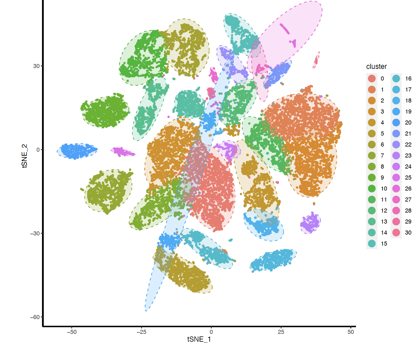
但是很方便可以自行调整。
文末友情推荐
要想真正入门生物信息学建议务必购买全套书籍,一点一滴攻克计算机基础知识,书单在:什么,生信入门全套书籍仅需160 。
如果大家没有时间自行慢慢摸索着学习,可以考虑我们生信技能树官方举办的学习班:
- 数据挖掘学习班第7期(线上直播3周,马拉松式陪伴,带你入门),原价4800的数据挖掘全套课程, 疫情期间半价即可抢购。
- 生信爆款入门-第9期(线上直播4周,马拉松式陪伴,带你入门),原价9600的生信入门全套课程,疫情期间3.3折即可抢购。
如果你课题涉及到转录组,欢迎添加一对一客服:详见:你还在花三五万做一个单细胞转录组吗?
号外:生信技能树知识整理实习生招募,长期招募,也可以简单参与软件测评笔记撰写,开启你的分享人生!另外,:绝大部分生信技能树粉丝都没有机会加我微信,已经多次满了5000好友,所以我开通了一个微信好友,前100名添加我,仅需150元即可,3折优惠期机会不容错过哈。我的微信小号二维码在:0元,10小时教学视频直播《跟着百度李彦宏学习肿瘤基因组测序数据分析》