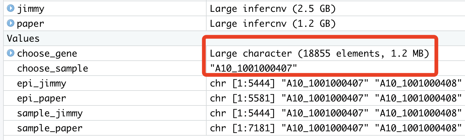
前面我提到了,我和文章都是取全部的上皮细胞,以及部分Fibroblasts和Endothelial_cells细胞来一起运行inferCNV流程。但是呢,自己的数据里面,是 366 genes and 7044 cells , 得到是CNV数量太少了(第18步写的是:Total CNV’s: 31 )计算量比较小,所以十几分钟就结束了。
而文章的这个数据集呢, Total CNV’s: 1229 太多了,耗费计算时间和资源有点过分了。它数据量:14869 genes and 7181 cells 其实不能选择 denoise=TRUE以及HMM=TRUE,都应该是用默认的FALSE即可。
首先把自己的数据集存为对象
rm(list=ls())
options(stringsAsFactors = F)
library(Seurat)
library(ggplot2)
library(infercnv)
expFile='expFile.txt'
groupFiles='groupFiles.txt'
geneFile='geneFile.txt'
infercnv_obj = CreateInfercnvObject(raw_counts_matrix=expFile,
 annotations_file=groupFiles,
 delim="\t",
 gene_order_file= geneFile,
 ref_group_names=c('ref-endo' ,'ref-fib')) ## 这个取决于自己的分组信息里面的
dim(infercnv_obj@expr.data)
dim(infercnv_obj@count.data)
dim(infercnv_obj@gene_order)
table(infercnv_obj@gene_order$chr)
infercnv_obj@reference_grouped_cell_indices
save(infercnv_obj,file='infercnv_obj_input_by_jimmy.Rdata')
然后读取文献的数据集
rm(list=ls())
options(stringsAsFactors = F)
library(Seurat)
library(ggplot2)
library(infercnv)
infercnv_obj = CreateInfercnvObject(raw_counts_matrix = "NI03_CNV_data_out_all_cells_raw_counts_largefile.txt",
 annotations_file = "NI03_CNV_cell_metadata_shuffle_largefile.txt",
 gene_order_file = "NI03_CNV_hg19_genes_ordered_correct_noXY.txt",
 ref_group_names = c("endothelial_normal", "fibroblast_normal"), delim = "\t")

paper=infercnv_obj
接着比较两个数据集
load('infercnv_obj_input_by_jimmy.Rdata')
jimmy=infercnv_obj
sample_jimmy=colnames(jimmy@expr.data)
sample_paper=colnames(paper@expr.data)
length(intersect(sample_jimmy,sample_paper))
# 这里我们的交集是 5388
epi_jimmy=colnames(jimmy@expr.data)[jimmy@observation_grouped_cell_indices$epi]
tmp=paper@observation_grouped_cell_indices
tmp=tmp[grepl('epi',names(tmp))]
epi_paper=colnames(paper@expr.data)[unique(unlist(tmp))]
length(intersect(epi_jimmy,epi_paper))
# 这里我们的交集是 5387

# 很有意思啊,我们选择的上皮细胞overlap非常好,但是我们选择的正常细胞,居然没有多少overlap
# 这里其实有一点点诡异,但是跟我们的主题无关。

choose_gene=intersect(rownames(jimmy@expr.data),
 rownames(paper@expr.data))
choose_sample=intersect(epi_jimmy,epi_paper)[1]
dat=cbind(jimmy@expr.data[choose_gene,choose_sample],
 paper@expr.data[choose_gene,choose_sample])
中间变量如下:
肉眼看了看作者数据集和我的差异,居然是—-
原来是我的表达量矩阵已经不再是纯粹的counts了,不是整数,而且居然是是被log后的,所以走inferCNV流程的时候,有一个步骤是 Removing genes from matrix as below mean expr threshold: 1, 绝大部分基因都这样被无情的删除了。
纠正后的inferCNV流程全部代码如下
rm(list=ls())
options(stringsAsFactors = F)
library(Seurat)
library(ggplot2)
load(file = 'first_sce.Rdata')
load(file = 'phe-of-first-anno.Rdata')
sce=sce.first
table(phe$immune_annotation)
sce@meta.data=phe
table(phe$immune_annotation,phe$seurat_clusters)
# BiocManager::install("infercnv")
library(infercnv)

epi.cells <- row.names(sce@meta.data)[which(phe$immune_annotation=='epi')]
length(epi.cells)
epiMat=as.data.frame(GetAssayData(subset(sce, slot='counts',
 cells=epi.cells)))

cells.use <- row.names(sce@meta.data)[which(phe$immune_annotation=='stromal')]
length(cells.use)
sce <-subset(sce, cells=cells.use)
sce
load(file = 'phe-of-subtypes-stromal.Rdata')
sce@meta.data=phe
DimPlot(sce, reduction = "tsne", group.by = "singleR")
table(phe$singleR)
fib.cells <- row.names(sce@meta.data)[phe$singleR=='Fibroblasts']
endo.cells <- row.names(sce@meta.data)[phe$singleR=='Endothelial_cells']
fib.cells=sample(fib.cells,800)
endo.cells=sample(endo.cells,800)
fibMat=as.data.frame(GetAssayData(subset(sce, slot='counts',
 cells=fib.cells)))
endoMat=as.data.frame(GetAssayData(subset(sce, slot='counts',
 cells=endo.cells)))

dat=cbind(epiMat,fibMat,endoMat)
groupinfo=data.frame(v1=colnames(dat),
 v2=c(rep('epi',ncol(epiMat)),
 rep('spike-fib',300),
 rep('ref-fib',500),
 rep('spike-endo',300),
 rep('ref-endo',500)))

library(AnnoProbe)
geneInfor=annoGene(rownames(dat),"SYMBOL",'human')
colnames(geneInfor)
geneInfor=geneInfor[with(geneInfor, order(chr, start)),c(1,4:6)]
geneInfor=geneInfor[!duplicated(geneInfor[,1]),]
length(unique(geneInfor[,1]))
head(geneInfor)
## 这里可以去除性染色体
# 也可以把染色体排序方式改变
dat=dat[rownames(dat) %in% geneInfor[,1],]
dat=dat[match( geneInfor[,1], rownames(dat) ),]
dim(dat)
expFile='expFile.txt'
write.table(dat,file = expFile,sep = '\t',quote = F)
groupFiles='groupFiles.txt'
head(groupinfo)
write.table(groupinfo,file = groupFiles,sep = '\t',quote = F,col.names = F,row.names = F)
head(geneInfor)
geneFile='geneFile.txt'
write.table(geneInfor,file = geneFile,sep = '\t',quote = F,col.names = F,row.names = F)

table(groupinfo[,2])

rm(list=ls())
options(stringsAsFactors = F)
library(Seurat)
library(ggplot2)
library(infercnv)
expFile='expFile.txt'
groupFiles='groupFiles.txt'
geneFile='geneFile.txt'
infercnv_obj = CreateInfercnvObject(raw_counts_matrix=expFile,
 annotations_file=groupFiles,
 delim="\t",
 gene_order_file= geneFile,
 ref_group_names=c('ref-endo' ,'ref-fib')) ## 这个取决于自己的分组信息里面的


## 直接走文献的代码:
infercnv_obj2 = infercnv::run(infercnv_obj,
 cutoff=1,
 out_dir= 'plot_out/inferCNV_output' ,
 cluster_by_groups=F, # cluster
 hclust_method="ward.D2", plot_steps=F)
差别就在GetAssayData函数,它获取Seurat对象里面的表达矩阵的时候加上了一个 slot=’counts’ 的参数,这样获取的就是原始从counts值。
如果数据量比较大
运行infercnv::run的时候,下面两个参数,都是默认值即可:
HMM参数 when set to True, runs HMM to predict CNV level (default: FALSE)
denoise If True, turns on denoising according to options below (default: FALSE)
如果你时间充裕,计算资源也充裕,就可以选择 denoise=TRUE以及HMM=TRUE。那么你会得到一个有意思的图表,如下:
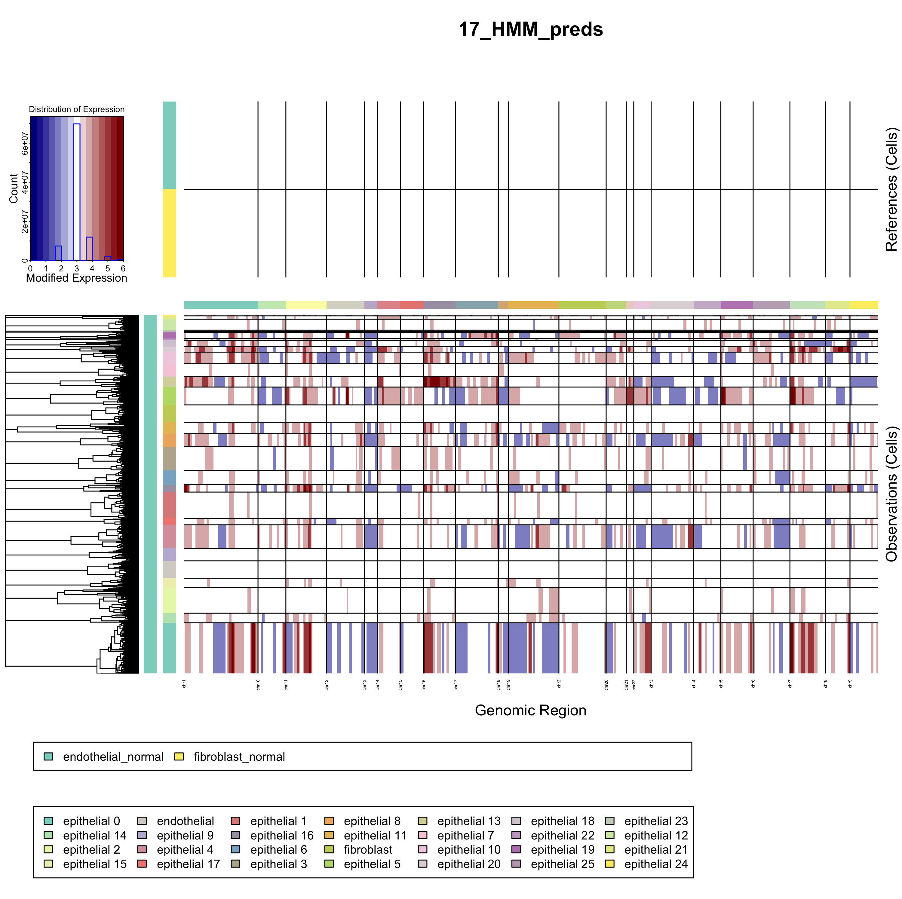
你可以自行比较这个图和文献里面的inferCNV结果图表。