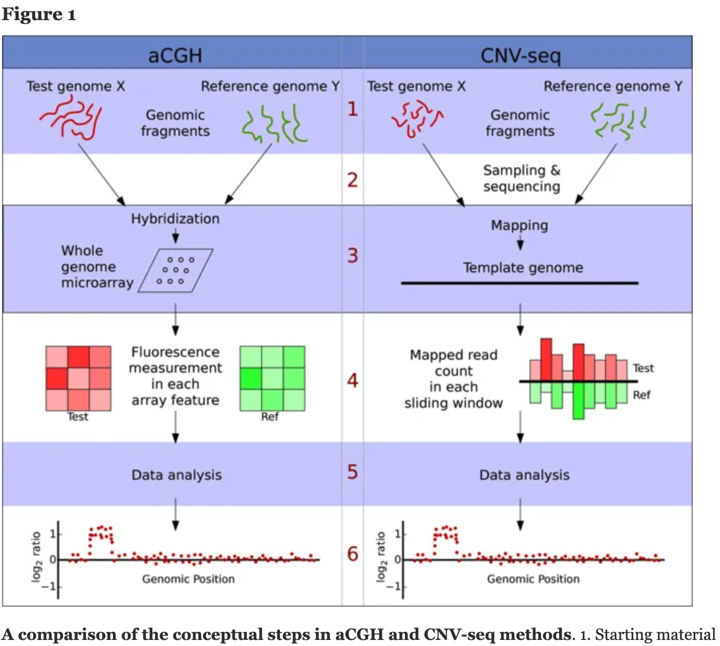
来自于2009发表在BMC Bioinformatics 的文章:CNV-seq, a new method to detect copy number variation using high-throughput sequencing ,这篇文章的重点是说明 CNV-seq 优于aCGH 在寻找拷贝数变异方面:
There are 121 CNV calls that made by CNV-seq but not aCGH and overlap with DGV data, suggesting that CNV-seq can detect CNV regions that were missed by aCGH.
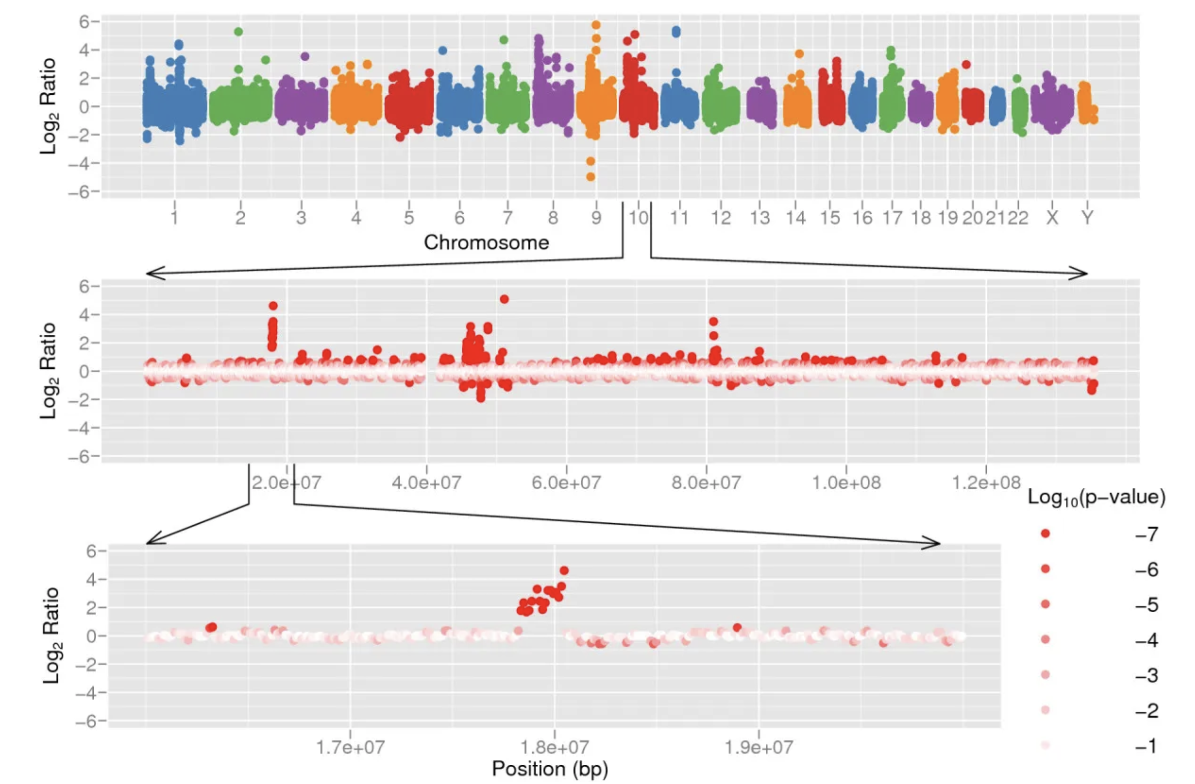
通过基因型log2ratio散点图展示了一个例子:One of these regions is shown in Figure 5 (bottom panel), a 238 kb region (copy number ratio 6:1, p = 0) containing two genes (FAM23B, MRC1L1) and one miRNA (hsa-mir-511-2)。就是说位于10号染色体的一个小片段,包括了两个基因和一个miRNA的238 kb 区域,就是一个被aCGH漏检的CNV片段。
其实就是一个基因型各个位点的测序的变异等位碱基比例(AF)散点图
Copy number variation detected by CNV-seq using shotgun sequence data from two individuals, Venter and Watson.
- The top panel shows a genome level log 2 ratio plot.
- The middle panel shows the plot for chromosome 10.
- The bottom panel shows detailed view of a CNV region in chromosome 10.
The red color gradient in the middle and bottom sections represents log10 p calculated on each of ratios.
肿瘤外显子数据也有类似的概念
在facets软件,有一个图我一直没有讲解清楚:
- Read depth ratio between tumor and normal gives information on total copy number.
- The variant (non-reference) allele frequency at heterozygous loci (germline variant allele frequency greater than 0.25 or less than 0.75) contain information on allelic imbalance.
- At each position, logR is dened by the log-ratio of total read depth in the tumor versus that in the normal and logOR is dened by the log-odds ratio of the variant allele count in the tumor versus in the normal.
拿到tumor和normal的测序深度和变异等位碱基深度
对tumor和normal两个样本都gvcf流程,拿到的vcf文件读入R里面,简单处理成为下表样式:
> dim(snpm)
[1] 552672 8
# 也就是拿到552672行信息,如下:
> head(snpm)
 CHROM POS gt dp ad gt dp ad
1 chr1 69270 1/1 2 2 1/1 8 8
2 chr1 69398 0/0 6 0 0/0 25 0
3 chr1 69410 0/0 7 0 0/0 25 0
4 chr1 69511 1/1 12 12 1/1 50 50
5 chr1 69849 ./. 0 0 0/0 4 0
6 chr1 69897 0/0 1 0 0/1 8 4
这个时候,需要对这个矩阵进行过滤,55万行的基因型信息还是挺多,一般来说,不需要考虑野生型位点,也就是保留’1/1’,’0/1’)这两种情况的位点。
> snpm=na.omit(snpm)
> ## only keep tumor or normal have mutations
> kp=snpm[,3] %in% c('1/1','0/1') | snpm[,6] %in% c('1/1','0/1')
> table(kp)
kp
 FALSE TRUE
473593 79056
> snpm=snpm[kp,]
> ## remove those show ./. positions
> kp=snpm[,3] == './.' | snpm[,6]== './.'
> print(table(!kp))

FALSE TRUE
 9494 69562
> snpm=snpm[!kp,c(1,2,4,5,7,8)]
> rcmat=snpm
> head(rcmat)
 CHROM POS dp ad dp.1 ad.1
1 chr1 69270 2 2 8 8
4 chr1 69511 12 12 50 50
6 chr1 69897 1 0 8 4
33 chr1 942335 4 4 9 9
34 chr1 942402 5 0 13 9
35 chr1 942451 5 5 11 11
> dim(rcmat)
[1] 69562 6
简单过滤后剩下不到7万的位点,这个时候绘图就差不多了。还可以进行测序深度的过滤,取决于你测序的实际情况,代码如下:
> rcmat=rcmat[rcmat[,3]>10,]
> rcmat=rcmat[rcmat[,5]>10,]
> rcmat$POS=as.numeric(rcmat$POS)
> dim(rcmat)
[1] 13224 6
> rcmat=na.omit(rcmat)
> colnames(rcmat)=c("Chromosome", "Position","NOR.DP","NOR.RD","TUM.DP","TUM.RD")
> rcmat[,1]=gsub('chr','',rcmat$Chrom)
> ## fit segmentation tree
> head(rcmat)
 Chromosome Position NOR.DP NOR.RD TUM.DP TUM.RD
4 1 69511 12 12 50 50
49 1 948245 11 11 35 35
91 1 961945 17 17 47 47
110 1 963956 11 6 52 18
143 1 973858 13 13 35 35
144 1 973862 13 6 35 19
> table(rcmat$Chromosome)

1 10 11 12 13 14 15 16 17 18 19 2 20 21 22 3
1444 657 768 725 286 408 489 469 588 262 663 1133 256 155 226 777
 4 5 6 7 8 9 X
 612 660 651 648 463 592 292
可以看到这个过滤有一点狠啦,剩下1.3万位点, 不过绘制散点图是绰绰有余啦。首先需要计算基因型各个位点的测序变异等位碱基比例(AF)在tumor和normal里面的差异,也就是log2ratio
rcmat$log2ratio=log2((rcmat[,4]/rcmat[,3])/(rcmat[,6]/rcmat[,5]))
plot(rcmat$log2ratio)
这个时候的图一定是丑爆的,如下:
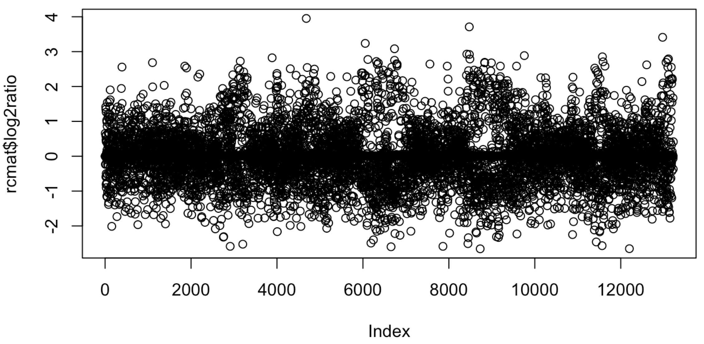
通常是对比得到的,比如一个tumor样本,在一个位点测到10个A和3个G,而其对应的normal样本在该位点是7个A和7个G,这个位点的参考基因组是G,所以呢,这个位点的normal的AF是0.5,而tumor的AF就有一点高,是0.77, 也就是说这个时候的AF的ratio是0.77/0.5=1.5啦,但是它被log2一下呢,就是log2(1.5)=0.6。
算起来有点复杂,不过现在都是机算啦,如果log2ratio是0,就说明这个位点在tumor和normal里面的AF是一致的。偏离0太多,就是所谓的CNV啦。
文末友情宣传
强烈建议你推荐给身边的博士后以及年轻生物学PI,多一点数据认知,让他们的科研上一个台阶:
- 底裤价转录组产品线(还送数据分析培训)(八九百一个样品)
- 三维基因组学分析实战培训班,线上直播课,2天仅需399(生信技能树粉丝特权价格)
- 生信技能树的2019年终总结 ,你的生物信息学成长宝藏
- 2020学习主旋律,B站74小时免费教学视频为你领路