Agilent的芯片同样也是扫描得到图片,然后图像处理(主要是Agilent Feature Extraction (AFE) 软件)得到信号值,但是值得注意的是,这个时候有两个信号值矩阵,分别是:the background matrix Eb as well as for the foreground matrix E.
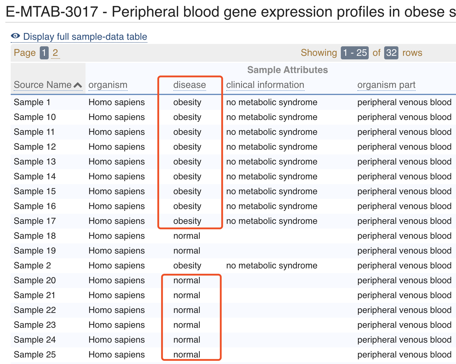
比如我们从ArrayExpress数据库下载一个E-MTAB-3017数据集,来源于文章:Peripheral blood gene expression profiles in obese subjects without metabolic syndrome
代码如下:
 library(ArrayExpress)
 ## getAE download all raw data for this study
 ## ArrayExpress just donwload the expressionSet
 rawset = ArrayExpress("E-MTAB-3017")
 # http://www.ebi.ac.uk/arrayexpress/experiments/E-MTAB-3017/
 ## it's not a AffyBatch object , but a NChannelSet for this study .
 ## for this platform the element names: E, Eb
 # the background matrix Eb as well as for the foreground matrix E.
 exprSet_Eb=assayDataElement(rawset,"Eb")
 exprSet_E=assayDataElement(rawset,"E")
 exprSet_E[1:4,1:4]
 exprSet_Eb[1:4,1:4]
既然是两个矩阵,所以分析需要格外注意,需要使用 Agi4x44PreProcess包,但是呢,这个包依赖旧版本的R和bioconductor,所以很麻烦:
 source("https://bioconductor.org/biocLite.R")
 biocLite("Agi4x44PreProcess")
很明显,我并不想耗费时间在这个上面,如果大家真的有必要处理这样的老旧数据,就需要自行摸索了,可以参考我前些天看到 https://www.ncbi.nlm.nih.gov/geo/query/acc.cgi?acc=GSE62117 的里面的详细数据处理步骤描述:
- The dataset was read into R and processed using the Agi4x44PreProcess package with options to use the AFE Processed Signal as foreground signal and BG Used signal as background adjusted signal.
- The data were then normalized by the quantile method using the limma function normalize Between Arrays.
- Probeset filtering was performed using the Agi4x44PreProcess filter method using AFE provided flags to identify features with quantification errors of the signal, reducing the 45,015 features on the Agilent Whole Human Genome Microarray 4x44K array by 38%, or 17,264 features.
- Residual technical batch effects were corrected using the ComBat method implemented in the SVA R package.
保守估计,如果确实有必要,5天内可以拿下这个数据分析!
这个同样的,也是学徒作业哈!使用使用 Agi4x44PreProcess包完成E-MTAB-3017数据集的表达矩阵获取。当然了,也可以根据分组,走一下差异分析标准代码:
走标准分析流程,火山图,热图,GO/KEGG数据库注释等等。这些流程的视频教程都在B站和GitHub了,目录如下:
- 第一讲:GEO,表达芯片与R
- 第二讲:从GEO下载数据得到表达量矩阵
- 第三讲:对表达量矩阵用GSEA软件做分析
- 第四讲:根据分组信息做差异分析
- 第五讲:对差异基因结果做GO/KEGG超几何分布检验富集分析
- 第六讲:指定基因分组boxplot指定基因list画热图
感兴趣可以细读表达芯片的公共数据库挖掘系列推文 ;