ncRNA芯片的一般分析流程

前面我们系统性的总结了circRNA的相关背景知识：

同样的策略，我们也可以应用到lncRNA的学习。所以昨天我们发布了：lncRNA的一些基础知识，那么接下来我们需要分享的就是lncRNA芯片的一般分析流程和lncRNA-seq数据的一般分析流程！

GEO数据库里面的lncRNA芯片平台很多

与circRNA芯片不同的是，GEO数据库里面的lncRNA芯片平台很多，毕竟已经是三五年前的热点了。

如果按照使用量排序，可以看到其实也就几百个数据集而已。

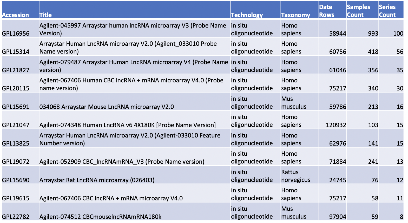
感兴趣的朋友可以点击进入查看详情。每个芯片平台的主页内容都是非常丰富的。

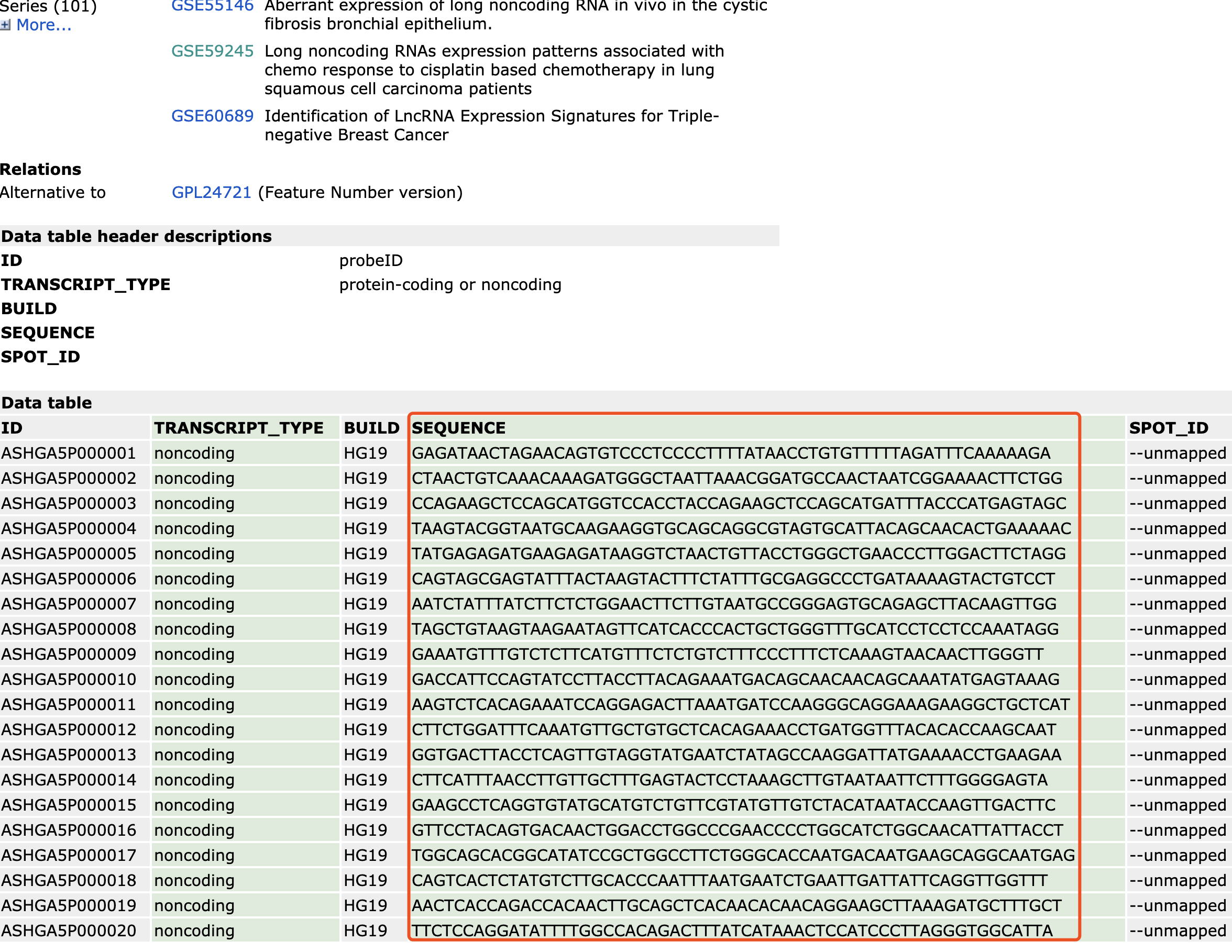
通常lncRNA芯片只有探针序列

比如：https://www.ncbi.nlm.nih.gov/geo/query/acc.cgi?acc=GPL16956 ，如下所示，有一百多个数据集都是使用的这个平台的芯片，但是可以看到，其GEO数据库主页里面，仅仅含有每个探针的碱基序列，并没有更丰富的lncRNA基因注释信息。

进入其中一个实例：https://www.ncbi.nlm.nih.gov/geo/query/acc.cgi?acc=GSE59245 我们可以学习一下，如何使用这样的lncRNA芯片。都是走标准分析流程，火山图，热图，GO/KEGG数据库注释等等。这些流程的视频教程都在B站和GitHub了，目录如下：

第一讲：GEO，表达芯片与R
第二讲：从GEO下载数据得到表达量矩阵
第三讲：对表达量矩阵用GSEA软件做分析
第四讲：根据分组信息做差异分析
第五讲：对差异基因结果做GO/KEGG超几何分布检验富集分析
第六讲：指定基因分组boxplot指定基因list画热图

仅仅是最后得到的差异分子，并不是以前的mRNA后面的基因名，而是miRNA，lncRNA，甚至circRNA的ID，看起来很陌生罢了。感兴趣可以细读表达芯片的公共数据库挖掘系列推文；

常规的表达量分析实验设计

来一个示例吧，这篇文章(Long noncoding RNAs expression patterns associated with chemo response to cisplatin based chemotherapy in lung squamous cell carcinoma patients. PLoS One 2014; PMID: 25250788) 使用的是 GPL16956 Agilent-045997 Arraystar human lncRNA microarray V3 (Probe Name Version)

分成2个组，然后走差异分析流程即可：

GSM1431249 69_PR
GSM1431250 80_PR
GSM1431251 83_PR
GSM1431252 141_PR
GSM1431253 164_PR
GSM1431254 165_PD
GSM1431255 169_PD
GSM1431256 175_PD
GSM1431257 177_PD
GSM1431258 198_PD

主要的结论就是根据什么阈值挑选到了多个上下调的lncRNAs基因：

Compared with the PD samples, 953 lncRNAs were consistently upregulated and 749 lncRNAs were downregulated consistently among the differentially expressed lncRNAs in PR samples (Fold Change≥2.0-fold, p <0.05).

因为是探索的是 lung squamous cell carcinoma 病人的chemo response to cisplatin，所以这个差异分析结果也正好跟”Nucleotide excision repair,” 等生物学功能富集。学徒作业：下载这个文章的这个数据集也走差异分析流程，并且进行GO/KEGG数据库功能富集注释看看是否与文章相符合。

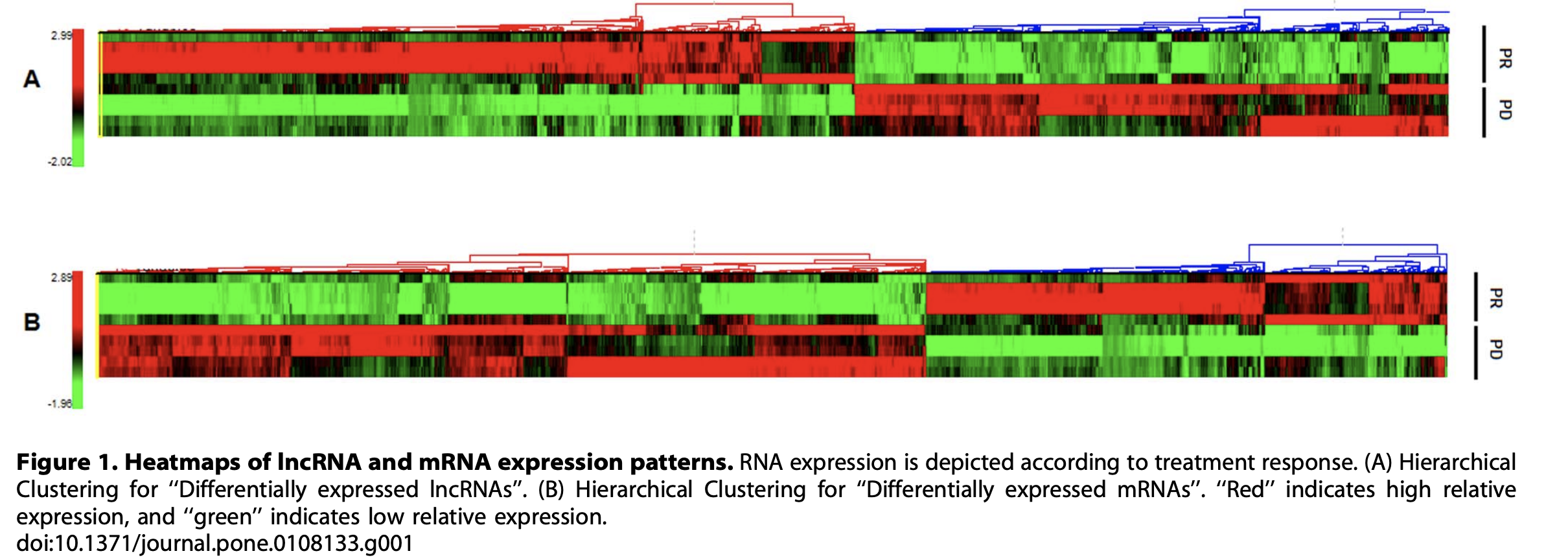
芯片里面是有 lncRNA 和 mRNA

就可以分开分析，分开走差异流程，分开富集分析，这样的话图表就多一点。比如文章就展示了两个热图，如下：

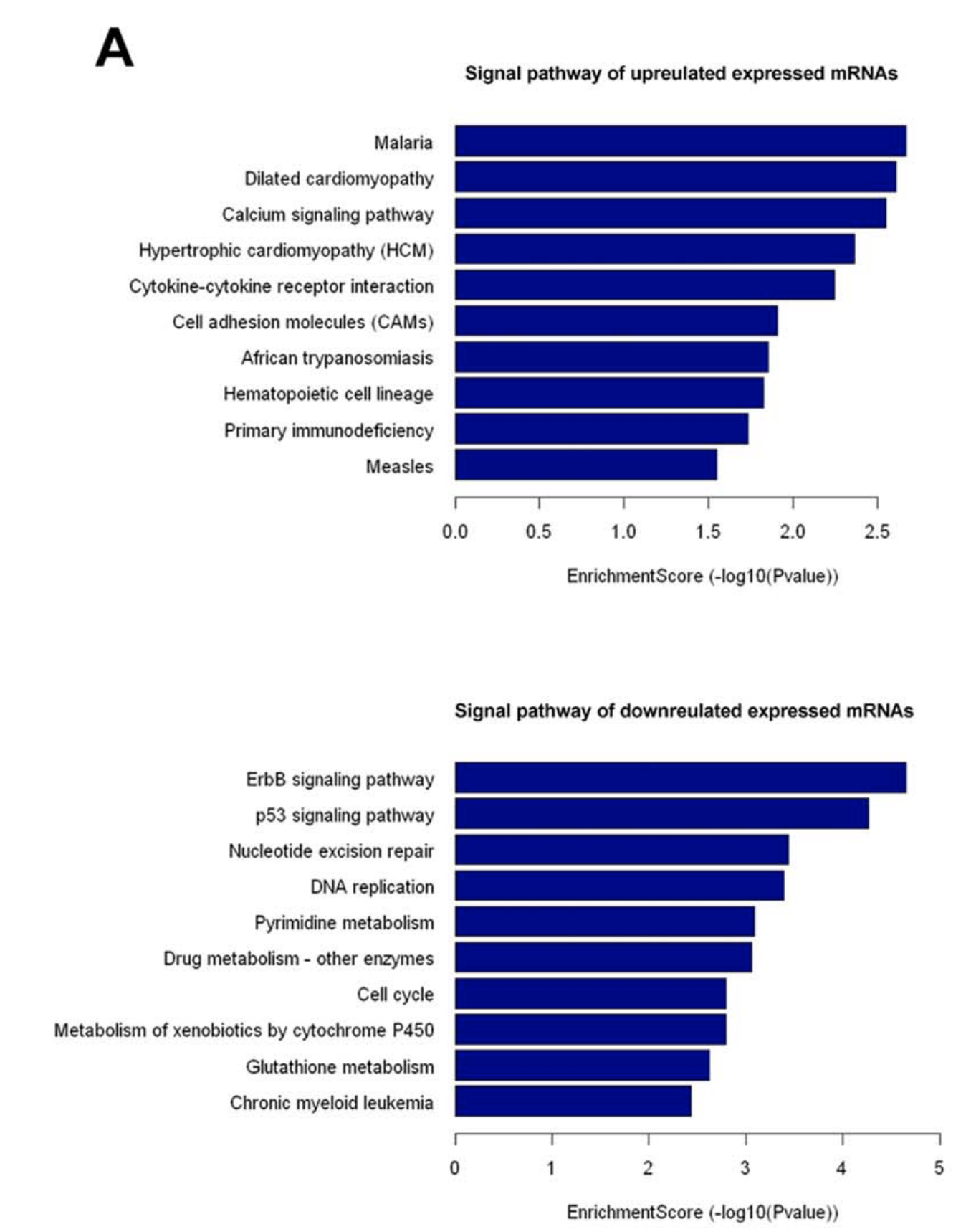
富集分析

可以看到，作者这里是把编码mRNA的基因分成统计学显著的上下调后，然后分开做KEGG数据库的超几何分布检验啦。可以看到，下调基因里面的功能排在第三的就是”Nucleotide excision repair,”符合作者的实验设计，肺癌的cisplatin耐药。

lncRNA芯片数据结果可以只是一个引子

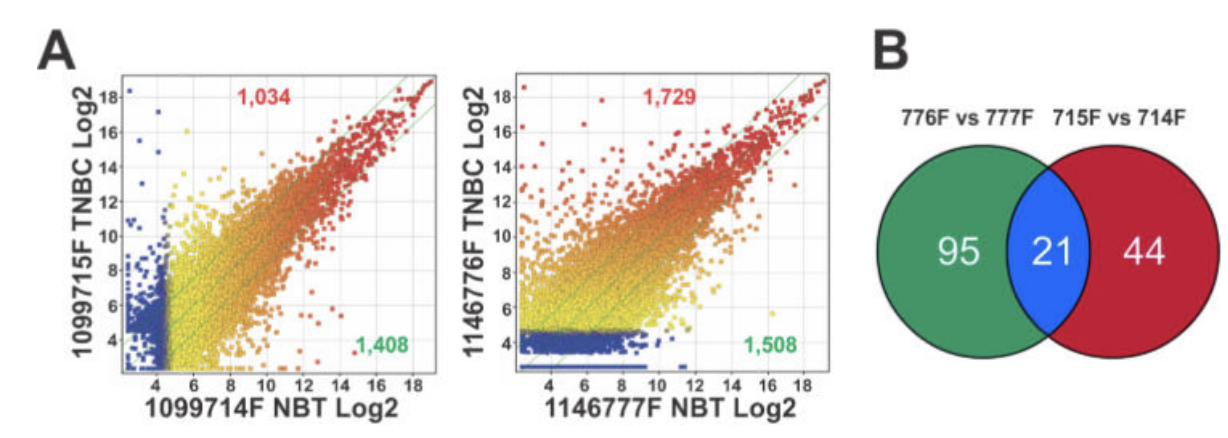
比如 GSE60689 Identification of LncRNA Expression Signatures for Triple-negative Breast Cancer ，文章是 lncRNA directs cooperative epigenetic regulation downstream of chemokine signals. Cell 2014 Nov PMID: 25416949 , 仅仅是4个样本，两个分组。

GSM1485226 Normal adjacent breast tissue [73]
GSM1485227 Infiltrating Ductal Carcinima of breast [73]
GSM1485228 Infiltrating Ductal Carcinima of breast [67]
GSM1485229 Normal adjacent breast tissue [67]

但是该做的分析一点都不会少，仍然是 Scatter plots of lncRNAs significantly up-regulated (red) or down-regulated (green) in two pairs of TNBC tissues compared to the matched adjacent normal tissues (NBT).

有趣的是，相当于这个文章的芯片其实是并没有生物学重复，两个病人独立的分析，然后取两个病人的差异基因的交集作为后续实验验证，因为这个cell文章，表达芯片的差异分析结果只是人家生物学故事的一个引子。

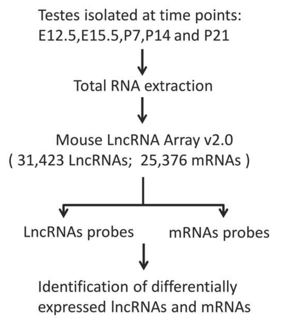
在小鼠的lncRNA芯片数据集例子

看数据集：GSE46896，其文章发表在一个很普通的杂志：Biol Reprod. 2013 Nov 7; 标题是：Expression profiling reveals developmentally regulated lncRNA repertoire in the mouse male germline 实验设计的很好，主要是分析太简陋了，生物学故事很一般。而且全文绘图都是Excel表格样式：

因为其分组比较多，所以可分析的点也会相应的多。

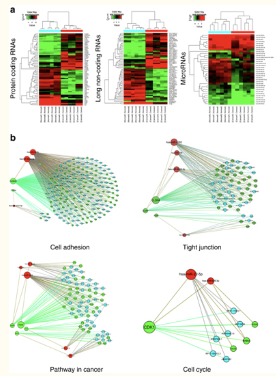
其实主要是共调控网络分析

共调控网络分析其实是公共数据库挖掘的一个很大众的方向，只要有两个表达矩阵，就可以分开独立走差异分析得到基因集，后续通过数据库进行关联，从而构建网络。

比如文章 Non-coding RNAs participate in the regulatory network of CLDN4 via ceRNA mediated miRNA evasion. Nat Commun 2017 Aug PMID: 28819095

GSM2643709 non-tumorous adjacent tissues_rep1
GSM2643710 non-tumorous adjacent tissues_rep2
GSM2643711 non-tumorous adjacent tissues_rep3
GSM2643712 non-tumorous adjacent tissues_rep4
GSM2643713 non-tumorous adjacent tissues_rep5
GSM2643714 non-tumorous adjacent tissues_rep6
GSM2643715 Gastric cancer tissues_rep1
GSM2643716 Gastric cancer tissues_rep2
GSM2643717 Gastric cancer tissues_rep3
GSM2643718 Gastric cancer tissues_rep4
GSM2643719 Gastric cancer tissues_rep5
GSM2643720 Gastric cancer tissues_rep6

就是分不同类型（ lncRNA 和 mRNA ）的基因，走差异分析流程，多个火山图，多个热图，最后挑选统计学显著的差异基因构建网络。所以需要加上miRNA芯片。

In an attempt to identify the regulatory networks of mRNA and ncRNAs in GC, six pairs of GC tissues and non-tumorous adjacent tissues were analyzed via microarray using the Human LncRNA+mRNA Array v3.0 together with the miRCURY LNATM microRNA Array.

类似的LncRNA + mRNA array 研究非常多，再比如文章：Long noncoding RNA expression profile reveals lncRNAs signature associated with extracellular matrix degradation in kashin-beck disease

LncRNA and mRNA expression profiling were performed using Agilent human lncRNA + mRNA array 4.0 platform (4 × 180 K), with each array containing approximately 41,000 lncRNA and 34,000 mRNA probes.

In this study, we identified 316 up-regulated and 631 down-regulated lncRNAs (≥ 2-fold change) in KBD chondrocytes

We also identified 232 up-regulated and 427 down-regulated mRNAs (≥ 2-fold change).

然后就针对具有统计学显著表达差异的LncRNA + mRNA 构建网络。

一个简单的例子

希望你安装一下AnnoProbe包，然后走下面的代码。

rm(list = ls())
library(AnnoProbe)
library(ggpubr)
suppressPackageStartupMessages(library(GEOquery))
getwd()
setwd('test/')
## download GSE95186 data
# https://www.ncbi.nlm.nih.gov/geo/query/acc.cgi?acc=GSE95186
# eSet=getGEO('GSE95186', destdir=".", AnnotGPL = F, getGPL = F)[[1]]
# 使用 GEO 中国区镜像进行加速

gset=AnnoProbe::geoChina('GSE95186')
gset
# check the ExpressionSet
eSet=gset[[1]]
probes_expr <- exprs(eSet);dim(probes_expr)
head(probes_expr[,1:4])
boxplot(probes_expr,las=2)
## pheno info
phenoDat <- pData(eSet)
head(phenoDat[,1:4])
# https://www.ncbi.nlm.nih.gov/pubmed/31430288

group_list=factor(c(rep('treat',3),rep('untreat',3)))
table(group_list)
eSet@annotation
# GPL15314 Arraystar Human LncRNA microarray V2.0 (Agilent_033010 Probe Name version)

GPL=eSet@annotation
# 选择 pipe 获取的是 冗余注释，也就是说一个探针很有可能会对应多个基因。
probes_anno <- idmap(GPL,type = 'pipe')
head(probes_anno)
probes_anno=probes_anno[probes_anno$probe_id %in% rownames(probes_expr),]
# 只需要表达矩阵里面有的探针的注释即可

length(unique(probes_anno$probe_id))
anno=annoGene(probes_anno$symbol,'SYMBOL')
head(anno)
pcs=probes_anno[probes_anno$symbol %in% anno[anno$biotypes=='protein_coding',1],]
nons=probes_anno[probes_anno$symbol %in% anno[anno$biotypes !='protein_coding',1],]
# 可以首先把探针拆分成为 protein_coding 与否
length(unique(pcs$probe_id))
length(unique(nons$probe_id))
# 可以看到仍然是有探针会被注释到多个基因，这个时候

pcs_expr <- probes_expr[pcs$probe_id,]
nons_expr <- probes_expr[nons$probe_id,]
boxplot(pcs_expr,las=2)
boxplot(nons_expr,las=2)
# 很容易看出来，非编码的这些基因的平均表达量，是低于编码的。

## 首先对编码基因的表达矩阵做差异分析
genes_expr <- filterEM(pcs_expr,pcs )
if(T){
 head(genes_expr)

library("FactoMineR")
 library("factoextra")
 dat.pca <- PCA(t(genes_expr) , graph = FALSE)
 dat.pca
 fviz_pca_ind(dat.pca,
 geom.ind = "point",
 col.ind = group_list,
 addEllipses = TRUE,
 legend.title = "Groups"
 )
 library(limma)
 design=model.matrix(~factor(group_list))
 design
 fit=lmFit(genes_expr,design)
 fit=eBayes(fit)
 DEG=topTable(fit,coef=2,n=Inf)
 head(DEG)
 ## visualization
 need_deg=data.frame(symbols=rownames(DEG), logFC=DEG$logFC, p=DEG$P.Value)
 deg_volcano(need_deg,1)
 deg_volcano(need_deg,2)

deg_heatmap(DEG,genes_expr,group_list)
 deg_heatmap(DEG,genes_expr,group_list,30)
}

### 然后对非编码的基因的表达矩阵做差异分析
genes_expr <- filterEM(nons_expr,nons )
if(T){
 head(genes_expr)

library("FactoMineR")
 library("factoextra")
 dat.pca <- PCA(t(genes_expr) , graph = FALSE)
 dat.pca
 fviz_pca_ind(dat.pca,
 geom.ind = "point",
 col.ind = group_list,
 addEllipses = TRUE,
 legend.title = "Groups"
 )
 library(limma)
 design=model.matrix(~factor(group_list))
 design
 fit=lmFit(genes_expr,design)
 fit=eBayes(fit)
 DEG=topTable(fit,coef=2,n=Inf)
 head(DEG)
 ## visualization
 need_deg=data.frame(symbols=rownames(DEG), logFC=DEG$logFC, p=DEG$P.Value)
 deg_volcano(need_deg,1)
 deg_volcano(need_deg,2)

deg_heatmap(DEG,genes_expr,group_list)
 deg_heatmap(DEG,genes_expr,group_list,30)
}

需要使用下面的代码自行下载安装我们的AnnoProbe包

library(devtools)
install_github("jmzeng1314/AnnoProbe")
library(AnnoProbe)

因为这个包里面并没有加入很多数据，所以理论上会比较容易安装，当然，不排除中国大陆少部分地方基本上连GitHub都无法访问。配合着详细的介绍：

因为这些包暂时托管在GitHub平台，但是非常多的朋友访问GitHub困难，尤其是我打包了好几百个GPL平台的注释信息后，我的GitHub包变得非常臃肿，大家下载安装困难，所以我重新写一个精简包。也在：芯片探针ID的基因注释以前很麻烦和：芯片探针序列的基因注释已经无需你自己亲自做了, 里面详细介绍了。最重要的是idmap函数，安装方法说到过：芯片探针序列的基因注释已经无需你自己亲自做了, 也有交流群，可以反馈使用过程的体验。

生信菜鸟团

欢迎去论坛biotrainee.com留言参与讨论，或者关注同名微信公众号biotrainee