接收到太多的粉丝求助,想下载个表达矩阵做一下数据挖掘偏偏第一步就卡住了,数据文件下载半天毫无动静,或者下载到99%就卡死了。如果我恰好在电脑旁,通常会帮忙下载后微云或者百度云传递给粉丝,但这毕竟不是长久之计,经过个把月的不懈努力,我终于把全部的GEO数据库里面的表达芯片数据都下载并且全部格式化处理成为r数据文件,并且购置一个2万块钱的腾讯云服务器来存放它们,供广大粉丝使用!
下载使用GEOmirror
有3种方法,如果都失败了,我就没办法说什么了。
Install the development version from Github:
library(devtools)
install_github("jmzeng1314/GEOmirror")
library(GEOmirror)
If it failed, just because your bad internet. You can also download this project directly into your computer, and then install it locally.
Or just use source function to load the codes of geoChina function, as below:
source('http://raw.githubusercontent.com/jmzeng1314/GEOmirror/master/R/geoChina.R')
What if all these 3 methods failed? I’m so sorry, what’ a pity that there’s no chance for you to use our GEOmirror !!
安装成功后,加载我们的R包会有一个提示,妈妈以后再也不用担心自己不知道怎么样致谢生信技能树团队啦!
这个就是官方致谢:在感恩节官宣!(文末有惊喜哈)
使用起来非常方便,就一句话,找到你的GSE数据集的ID,传给我们的函数即可:
use it to download GEO dataset, as below :
eSet=geoChina('GSE1009')
eSet=geoChina('GSE27533')
eSet=geoChina('GSE95166')
举一个简单的例子
Once you download the ExpressionSet of GEO dataset, you can access the expression matrix and phenotype data:
## download GSE95166 data
# https://www.ncbi.nlm.nih.gov/geo/query/acc.cgi?acc=GSE95166
#eSet=getGEO('GSE95166', destdir=".", AnnotGPL = F, getGPL = F)[[1]]
library(GEOmirror)
eSet=geoChina('GSE95166')
eSet
eSet=eSet[[1]]

probes_expr <- exprs(eSet);dim(probes_expr)
head(probes_expr[,1:4])
boxplot(probes_expr,las=2)

## pheno info
phenoDat <- pData(eSet)
head(phenoDat[,1:4])
# https://www.ncbi.nlm.nih.gov/pubmed/31430288

groupList=factor(c(rep('npc',4),rep('normal',4)))
table(groupList)
eSet@annotation
# GPL15314 Arraystar Human LncRNA microarray V2.0 (Agilent_033010 Probe Name version)
对于这一点表达矩阵数据集,我们可以看看PCA图,火山图以及热图:
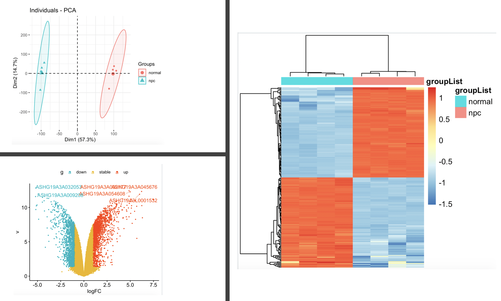
代码如下:
genes_expr=probes_expr
library("FactoMineR")
library("factoextra")
dat.pca <- PCA(t(genes_expr) , graph = FALSE)
dat.pca
fviz_pca_ind(dat.pca,
 geom.ind = "point",
 col.ind = groupList,
 addEllipses = TRUE,
 legend.title = "Groups"
)
library(limma)
design=model.matrix(~factor(groupList))
design
fit=lmFit(genes_expr,design)
fit=eBayes(fit)
DEG=topTable(fit,coef=2,n=Inf)
head(DEG)
# We observed that 2107 lncRNAs were upregulated
# while 2090 lncRNAs were downregulated by more than 2-fold,
# NKILA among these downregulated lncRNAs (Fig 1A, GSE95166).

## for volcano plot
df=DEG
attach(df)
df$v= -log10(P.Value)
df$g=ifelse(df$P.Value>0.05,'stable',
 ifelse( df$logFC >1,'up',
 ifelse( df$logFC < -1,'down','stable') )
)
table(df$g)
df$name=rownames(df)
head(df)
library(ggpubr)
ggpubr::ggscatter(df, x = "logFC", y = "v", color = "g",size = 0.5,
 label = "name", repel = T,
 label.select =head(rownames(df)),
 palette = c("#00AFBB", "#E7B800", "#FC4E07") )
detach(df)

x=DEG$logFC
names(x)=rownames(DEG)
cg=c(names(head(sort(x),100)),
 names(tail(sort(x),100)))
cg
library(pheatmap)
n=t(scale(t(genes_expr[cg,])))
n[n>2]=2
n[n< -2]= -2
n[1:4,1:4]
ac=data.frame(groupList=groupList)
rownames(ac)=colnames(n)
pheatmap(n,show_colnames =F,show_rownames = F,
 annotation_col=ac)
实际上,这个时候,我们需要把探针的ID转换为基因名字,进行后续分析,不过这个比较复杂超出了本文范围,感兴趣的看:(重磅!价值一千元的R代码送给你)芯片探针序列的基因组注释
是不是很激动,想试试看
同样的代码,你可以处理自己的数据集哦。
因为功能非常简单,just a replacement of getGEO function from GEOquery package.
所以是不会有bug的,但是,也许大家在使用的过程有新的需求,我可以酌情根据时间来开发增加功能,感兴趣可以进入我们的交流群:4年前的TCGA重磅资料你学了吗
当然了,表达芯片的公共数据库挖掘系列更多教程,见推文 ;