表达芯片数据处理教程,早在2016年我就系统性整理了发布在生信菜鸟团博客:http://www.bio-info-trainee.com/2087.html 配套教学视频在B站:https://www.bilibili.com/video/av26731585/ 代码都在:https://github.com/jmzeng1314/GEO 早期目录如下:
- 第一讲:GEO,表达芯片与R
- 第二讲:从GEO下载数据得到表达量矩阵
- 第三讲:对表达量矩阵用GSEA软件做分析
- 第四讲:根据分组信息做差异分析
- 第五讲:对差异基因结果做GO/KEGG超几何分布检验富集分析
- 第六讲:指定基因分组boxplot指定基因list画热图
- 第七讲:根据差异基因list获取string数据库的PPI网络数据
- 第八讲:PPI网络数据用R或者cytoscape画网络图
- 第九讲:网络图的子网络获取
- 第十讲:hug genes如何找
但并不是万能的,即使是表达芯片,也有一些是我的知识盲区,主要是因为没有时间去继续探索整理写教程,毕竟大家都不支持我写教程,没有人打赏或者留言鼓励我!
不过最近学徒问到了[HTA-2_0] Affymetrix Human Transcriptome Array 2.0芯片的事情,其实挺麻烦的,首先需要搞清楚下面3个平台的差异:
- GPL17586 [HTA-2_0] Affymetrix Human Transcriptome Array 2.0 [transcript (gene) version]
- GPL19251 [HuGene-2_0-st] Affymetrix Human Gene 2.0 ST Array [probe set (exon) version]
- GPL16686 [HuGene-2_0-st] Affymetrix Human Gene 2.0 ST Array [transcript (gene) version]
如果是芯片cel原始数据处理
那么看我的教程 你要挖的公共数据集作者上传了错误的表达矩阵肿么办(如何让高手心甘情愿的帮你呢?) 里面有提到:
# BiocManager::install(c( 'oligo' ),ask = F,update = F)
library(oligo)
# BiocManager::install(c( 'pd.hg.u133.plus.2' ),ask = F,update = F)
library(pd.hg.u133.plus.2)

dir='~/Downloads/GSE84571_RAW/'
 od=getwd()
 setwd(dir)
 celFiles <- list.celfiles(listGzipped = T)
 celFiles
 affyRaw <- read.celfiles( celFiles )
 setwd(od)
 eset <- rma(affyRaw)
 eset
 # http://math.usu.edu/jrstevens/stat5570/1.4.Preprocess_4up.pdf
 save(eset,celFiles,file = f)
 # write.exprs(eset,file="data.txt")
当然了,你没有R基础是看不懂的哈。
如果是芯片注释到基因
也是很简单
 library(GEOquery)
 #Download GPL file, put it in the current directory, and load it:
 gpl <- getGEO('GPL19251', destdir=".")
 colnames(Table(gpl))
 head(Table(gpl)[,c(1,10)]) ## you need to check this , which column do you need
 probe2gene=Table(gpl)[,c(1,10)]
 head(probe2gene)
 library(stringr)
 probe2gene$symbol=trimws(str_split(probe2gene$gene_assignment,'//',simplify = T)[,2])
 plot(table(table(probe2gene$symbol)),xlim=c(1,50))
 head(probe2gene)
 save(probe2gene,file='probe2gene.Rdata')
不同平台, 就替换GPL,然后自行看输入输出判断一下即可,也需要R基础啦。
如果是差异分析
当然了也可以直接修改我的代码,不过这个HTA2.0芯片比较麻烦的在于,基于exon和基于transcript的有一点点区别,因为基于exon理论上可以获取不同剪切体的表达量差异的,虽然实际上很少有人愿意去探索。
发表在 BMC Genomics. 2017; 文章 RNA sequencing and transcriptome arrays analyses show opposing results for alternative splicing in patient derived samples 就提到过。
更麻烦的是,因为这个芯片记录35万个外显子,这样矩阵就非常大, 都可以与根据illumina的450K甲基化芯片媲美啦!
可以看到,大量的基因有着1-30个探针,如下:
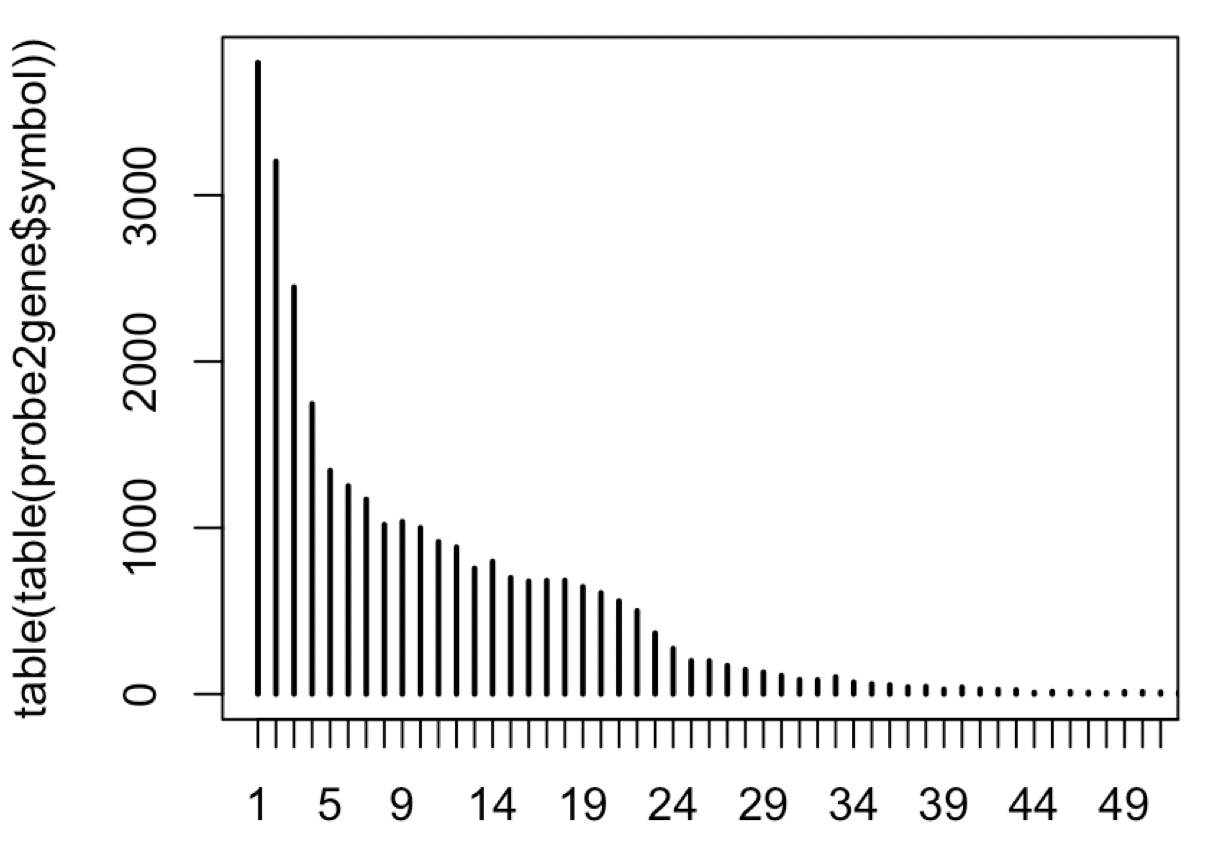
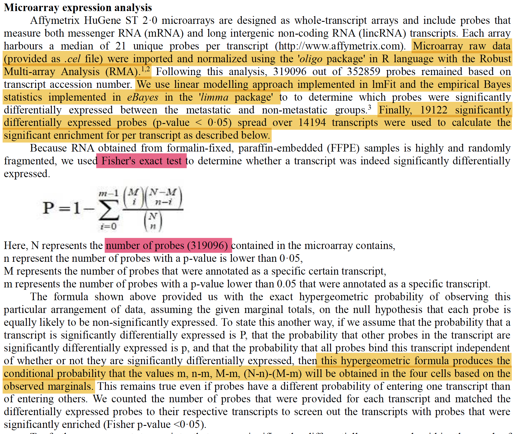
所以有文章采取非常特殊的差异分析策略:
最后一个作业
大家可以拿 https://www.ncbi.nlm.nih.gov/geo/query/acc.cgi?acc=GSE118222 数据集,测试看看,走我给大家的代码,得到PCA,热图,火山图,看看是否合理。
GSM3321243 LNCaP EtOH rep 1
GSM3321244 LNCaP EtOH rep 2
GSM3321245 LNCaP DHT rep 1
GSM3321246 LNCaP DHT rep 2
GSM3321247 LNCaP ABT-DHT rep 1
GSM3321248 LNCaP ABT-DHT rep 2
GSM3321249 C4-2 DMSO rep 1
GSM3321250 C4-2 DMSO rep 2
GSM3321251 C4-2 ABT rep 1
GSM3321252 C4-2 ABT rep 2