多个样本单细胞转录组数据整合算法以 mutual nearest neighbors (MNNs)和canonical correlation analysis (CCA) 最为出名,见 详细介绍多个单细胞转录组样本的数据整合之CCA-Seurat包
这里我们使用一下scran包的 mutual nearest neighbors (MNNs)方法吧,主要就是读文档而已:https://bioconductor.org/packages/release/bioc/vignettes/scran/inst/doc/scran.html
首先模拟一个表达矩阵
这里简单的R矩阵使用scran包的SingleCellExperiment函数即可构建SingleCellExperiment对象:
library(scran)
ngenes <- 10000
ncells <- 200
mu <- 2^runif(ngenes, -1, 5)
gene.counts <- matrix(rnbinom(ngenes*ncells, mu=mu, size=10), nrow=ngenes)
sce <- SingleCellExperiment(list(counts=gene.counts))
sce <- computeSumFactors(sce)
sce <- normalize(sce)
然后模拟一下批次效应
同样也是很简单的一个随机数:
b1 <- sce
b2 <- sce
# Adding a very simple batch effect.
logcounts(b2) <- logcounts(b2) + runif(nrow(b2), -1, 1)
combined <- cbind(b1, b2)
combined$batch <- gl(2, ncol(b1))
library(scater)
plotPCA(combined, colour_by="batch") + ggtitle("Without correction")
可以看到批次效应清晰可见:
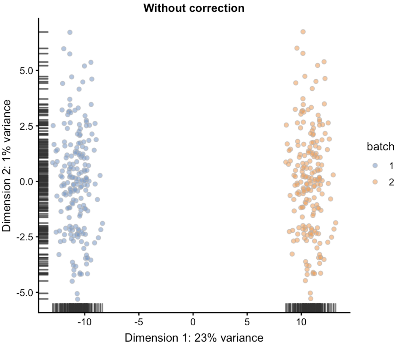
这里采用的是scater包的plotPCA函数对SingleCellExperiment这样的对象之间PCA运算并且可视化。
接着使用scater包的fastMNN去除批次效应
out <- fastMNN(b1, b2)
dim(out$corrected)
out$batch
reducedDim(combined, "corrected") <- out$correct
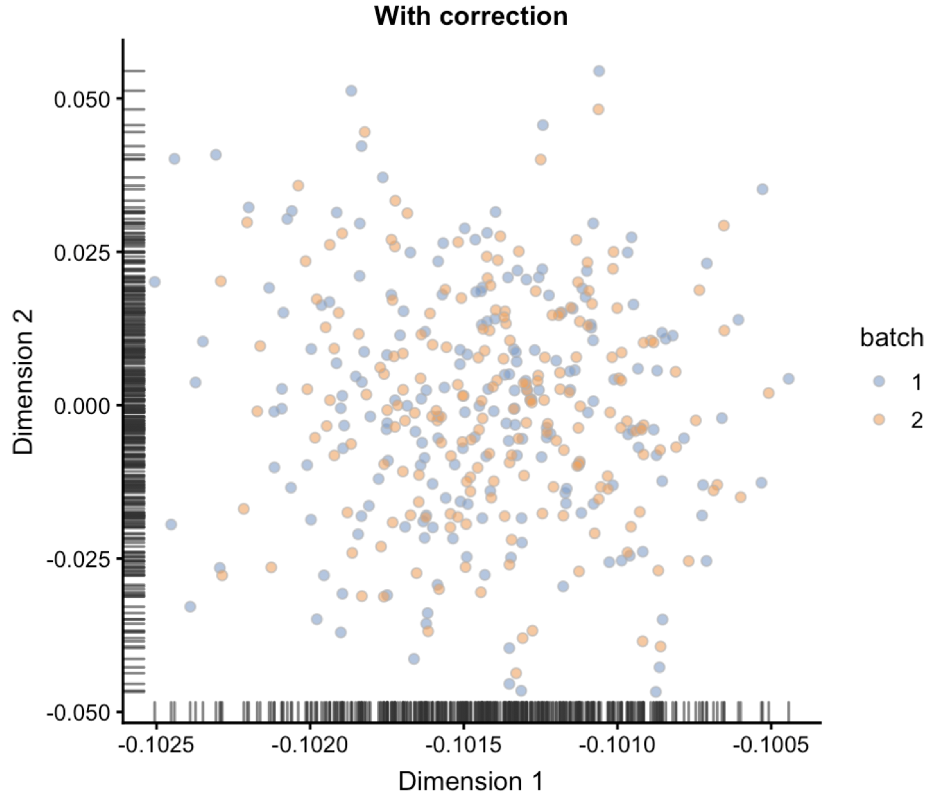
plotReducedDim(combined, "corrected", colour_by="batch") + ggtitle("With correction")
可以非常清楚的看到批次效应被去除了:
在scRNAseq包的表达矩阵测试
这个包内置的是 Pollen et al. 2014 数据集,人类单细胞细胞,分成4类,分别是 pluripotent stem cells 分化而成的 neural progenitor cells (“NPC”) ,还有 “GW16” and “GW21” ,“GW21+3” 这种孕期细胞,理解这些需要一定的生物学背景知识,如果不感兴趣,可以略过。
这个R包大小是50.6 MB,下载需要一点点时间,先安装加载它们。
这个数据集很出名,截止2019年1月已经有近400的引用了,后面的人开发R包算法都会在其上面做测试,比如 SinQC 这篇文章就提到:We applied SinQC to a highly heterogeneous scRNA-seq dataset containing 301 cells (mixture of 11 different cell types) (Pollen et al., 2014).
不过本例子只使用了数据集的4种细胞类型而已,因为 scRNAseq 这个R包就提供了这些,完整的数据是 23730 features, 301 samples, 地址为https://hemberg-lab.github.io/scRNA.seq.datasets/human/tissues/ , 这个网站非常值得推荐,简直是一个宝藏。
这里面的表达矩阵是由 RSEM (Li and Dewey 2011) 软件根据 hg38 RefSeq transcriptome 得到的,总是130个文库,每个细胞测了两次,测序深度不一样。
首先拿出表达矩阵构建两个SingleCellExperiment对象
library(scRNAseq)
## ----- Load Example Data -----
data(fluidigm)
ct <- floor(assays(fluidigm)$rsem_counts)
ct[1:4,1:4]
sample_ann <- as.data.frame(colData(fluidigm))
table(sample_ann$Coverage_Type)
table(sample_ann$Biological_Condition)

kp=sample_ann$Coverage_Type=='High'
sce <- SingleCellExperiment(
 assays = list(counts = ct[,kp]),
 colData = sample_ann[kp,]
)
sce
sce <- computeSumFactors(sce)
sce <- normalize(sce)
b1 <- sce
kp=sample_ann$Coverage_Type=='Low'
sce <- SingleCellExperiment(
 assays = list(counts = ct[,kp]),
 colData = sample_ann[kp,]
)
sce <- computeSumFactors(sce)
sce <- normalize(sce)
b2 <- sce
然后绘制处理前的PCA图
combined <- cbind(b1, b2)
combined$batch <- gl(2, ncol(b1))
library(scater)
plotPCA(combined, colour_by="batch",shape_by='Biological_Condition') + ggtitle("Without correction")
可以看到,不同测序深度的两类细胞分的非常开,就是技术差异批次效应:
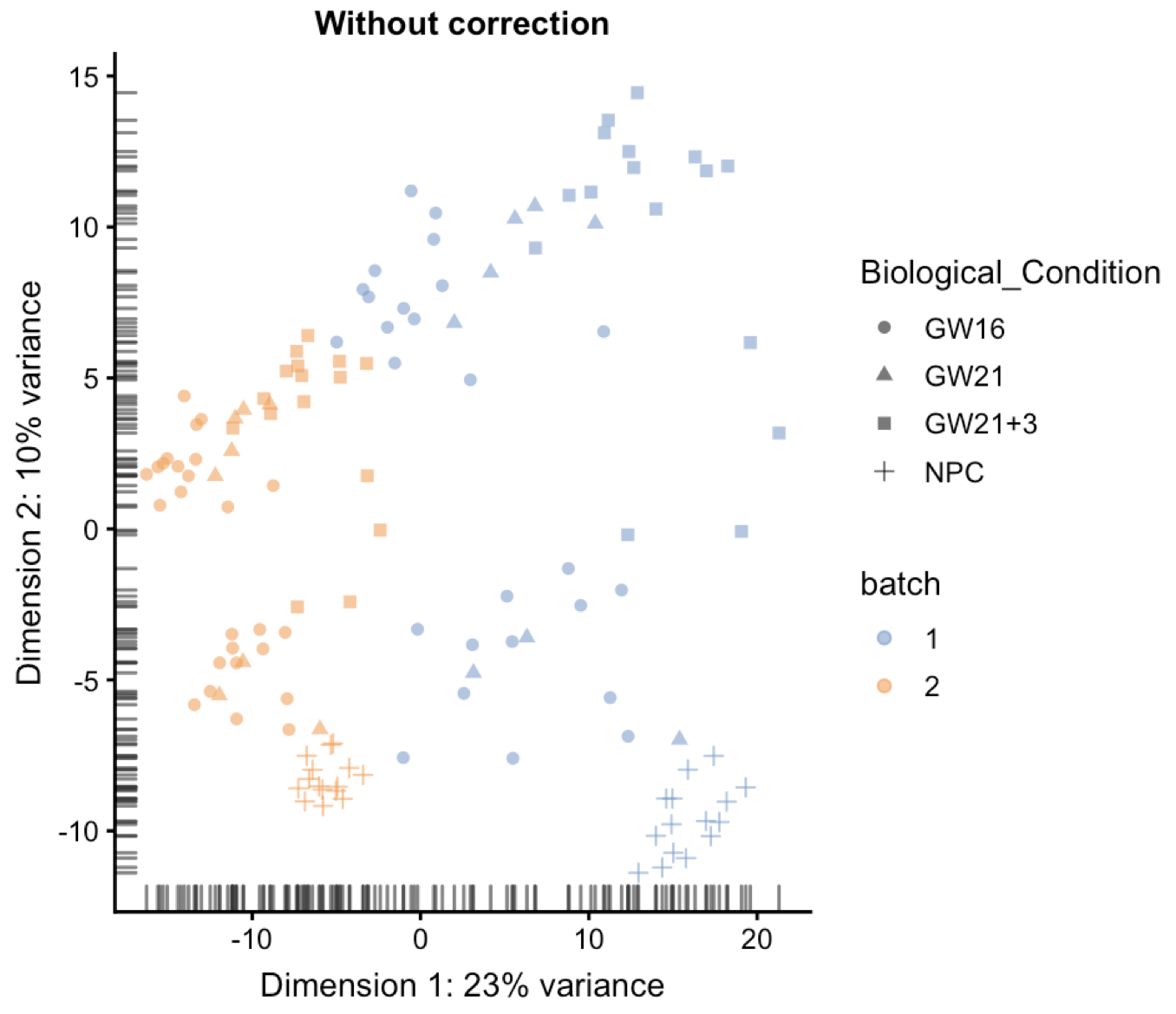
上图中的NPC细胞,使用+表示的那些点,可以看到不同颜色的左右分很开,仅仅是因为他们的文库测序大小不一样。
使用scater包的fastMNN去除批次效应
out <- fastMNN(b1, b2)
dim(out$corrected)
out$batch
reducedDim(combined, "corrected") <- out$correct
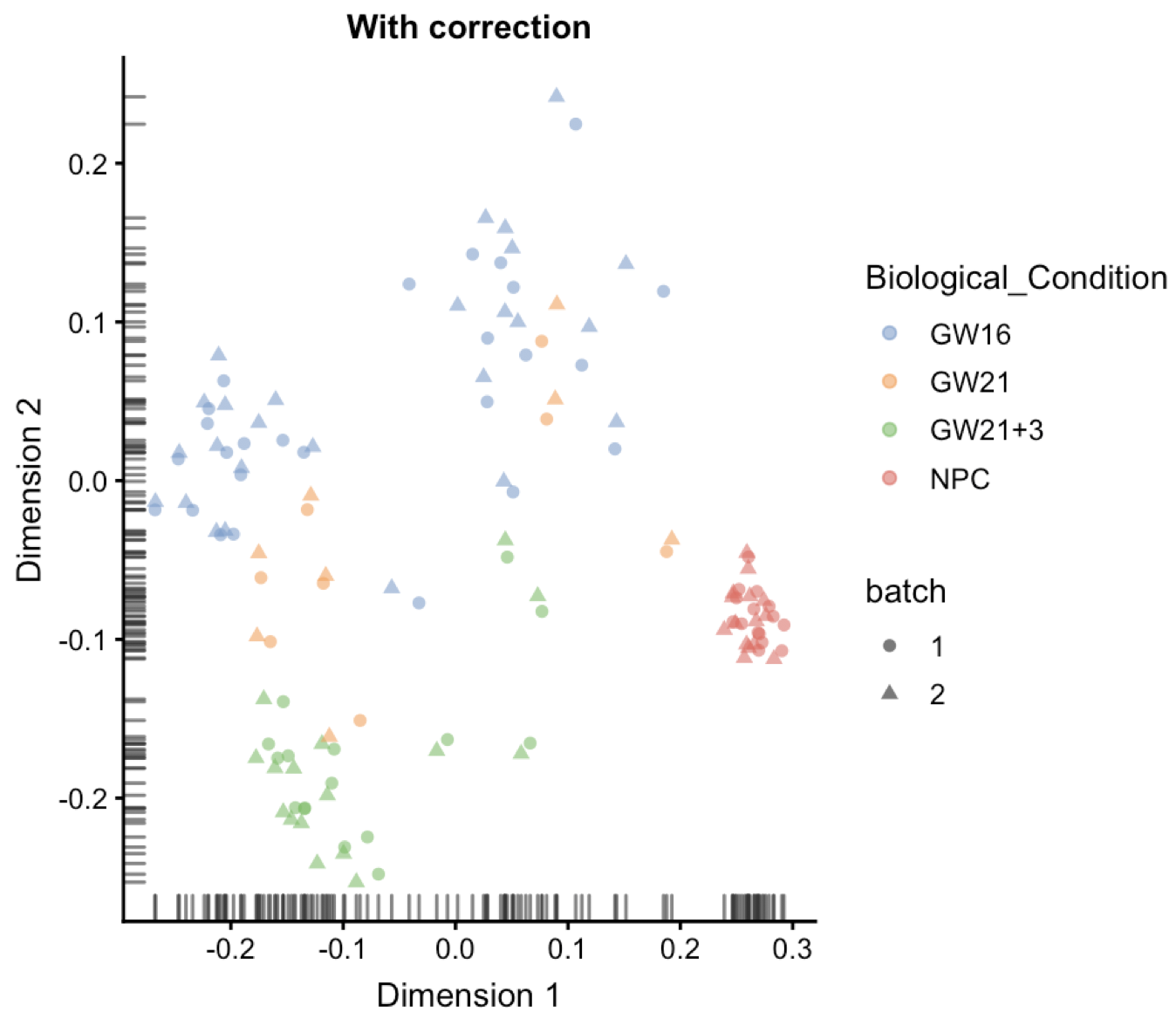
plotReducedDim(combined, "corrected", shape_by ="batch",colour_by='Biological_Condition') + ggtitle("With correction")
可以看到大不一样,这个时候的NPC,就是下图深红色的,可以看到不同batch聚集的非常近,效果很棒!
后记
其实scran这个包,我们介绍最多的是Cell cycle phase assignment功能,也就是推断细胞周期。