发表于: 2015 Dec 4. doi: 10.1038/ncomms9971
众所周知,肿瘤样品纯度是很有限的,包括围绕在肿瘤细胞周围的各种免疫细胞,还有肿瘤微环境其它细胞。
作者团队在这里对TCGA计划的21种癌症的超过10000个样本系统性的分析了肿瘤纯度
数据来源
We obtained gene expression profiles (RNA-seqV2), DNA methylation profiles (HumanMethylation450) and immunohistochemistry (IHC) analysis for 9,364 tumour samples and 1,958 adjacent normal samples across 21 solid tumour types from the TCGA repository
比较4种估算肿瘤纯度的方法
这里采用4种方法:
- ESTIMATE, which uses gene expression profiles of 141 immune genes and 141 stromal genes6;
- ABSOLUTE, which uses somatic copy-number data (estimations were available for only 11 cancer types)7;
- LUMP (leukocytes unmethylation for purity), which averages 44 non-methylated immune-specific CpG sites (Supplementary Fig. 1 and Methods);
- IHC, as estimated by image analysis of haematoxylin and eosin stain slides produced by the Nationwide Children’s Hospital Biospecimen Core Resource.
三种DNA, RNA and methylation-based方法估算的肿瘤纯度一致性比较高,但是都跟IHC的差异比较大。
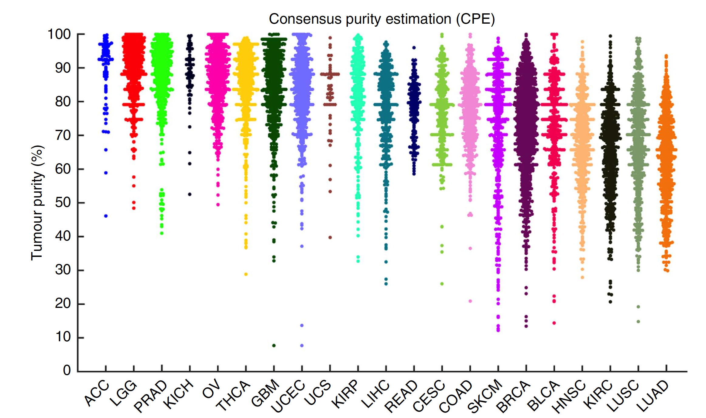
结果文件都是在:Tumor purity estimates for TCGA samples. Tumor purity estimates according to four methods and the consensus method for all TCGA samples with available data.
Click here to view.(540K, xlsx) 下载后可以自行作图进行可视化,粗略看起来肿瘤纯度平均值在0.8左右,如下图:
不同肿瘤纯度方法的归一化
全称是:consensus measurement of purity estimations (CPE)
这里的归一化很简单, CPE is the median purity level after normalizing levels from all methods to give them equal means and s.d.’s (75.3±18.9%).
后续分析都使用的是CPE值,具有替代性。
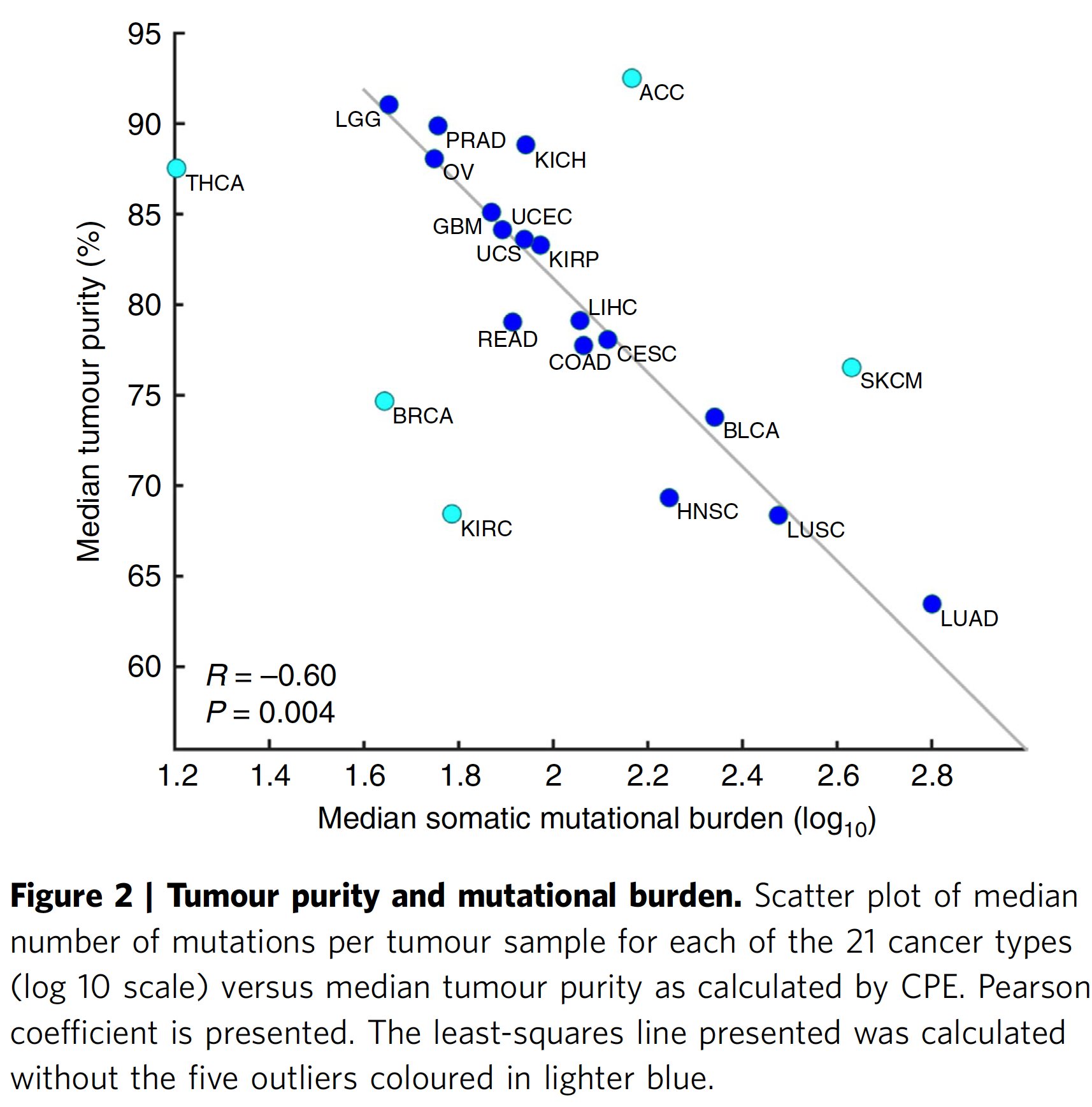
然后作者通过分析发现 median purity levels and median mutational burden 具有非常好的相关性,如下:
肿瘤纯度和其它临床信息的关联性
这里作者这里了722种临床信息,其中299种是不同肿瘤种类特有的,最后发现sex, age, ethnicity, alcohol use and smoking 这些指标跟肿瘤纯度无关,不过只要是统计分析,或多或少都会得到一些显著性指标的,作者毫不例外的在正文描述了那些显著性的。
当然,少不了的是生存分析结果。校正肿瘤纯度对其它NGS组学分析结果的影响
比如之前的表达数据的聚类,看看是否聚类结果其实是受到了肿瘤纯度的摆布。
是否有些基因的表达量是跟肿瘤纯度相关的。
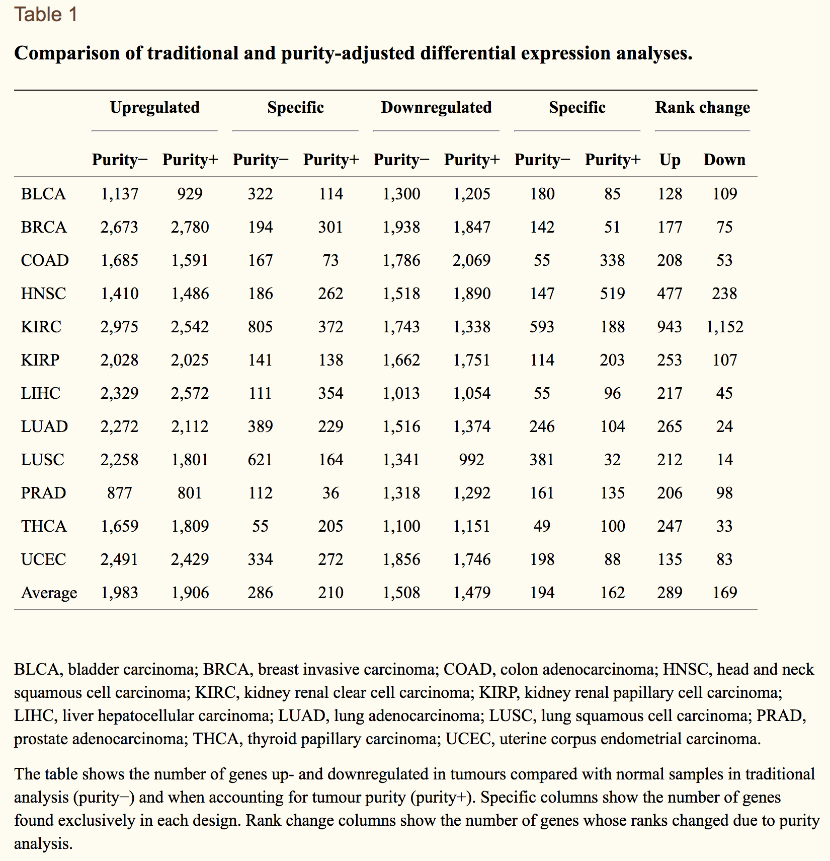
是否肿瘤纯度会影响差异分析结果,所以作者使用DESeq2包来引入纯度这个变量进行校正。
可以参考去除batch effect的用法,这里的肿瘤纯度这个连续变量可以根据高低进行分组设置为离散变量即可。
使用limma包的removeBatchEffect来处理。
countData: 表达矩阵
colData: 样品分组信息表
design: 实验设计信息,batch和conditions必须是colData中的一列dds <- DESeqDataSetFromMatrix(countData = data, colData = sample, design= ~ batch + conditions) dds <- DESeq(dds) ## 数据集小于30 -> rlog,大数据集 -> VST。 rld <- rlog(dds, blind=FALSE) rlogMat <- assay(rld) rlogMat <- limma::removeBatchEffect(rlogMat, c(sample$batch)) #VST, remove batch effect, then plotPCA: vsd <- vst(dds) plotPCA(vsd, "batch") assay(vsd) <- limma::removeBatchEffect(assay(vsd), vsd$batch) plotPCA(vsd, "batch")代码比较简单,思路最重要。
DESeq2为count数据提供了两类变换方法,使得不同均值的方差趋于稳定:regularized-logarithm transformation or rlog(Love, Huber, and Anders 2014)和variance stabilizing transformation(VST)(Anders and Huber 2010)用于处理含有色散平均趋势负二项数据。
结果如下:
此文章完全是数据分析,值得学习。